If you’ve ever had to sum up items across many different sheets, then you know it can be a real pain when there are a lot of sheets. This trick will make it super easy.
Get the example workbook with the above link to follow along.

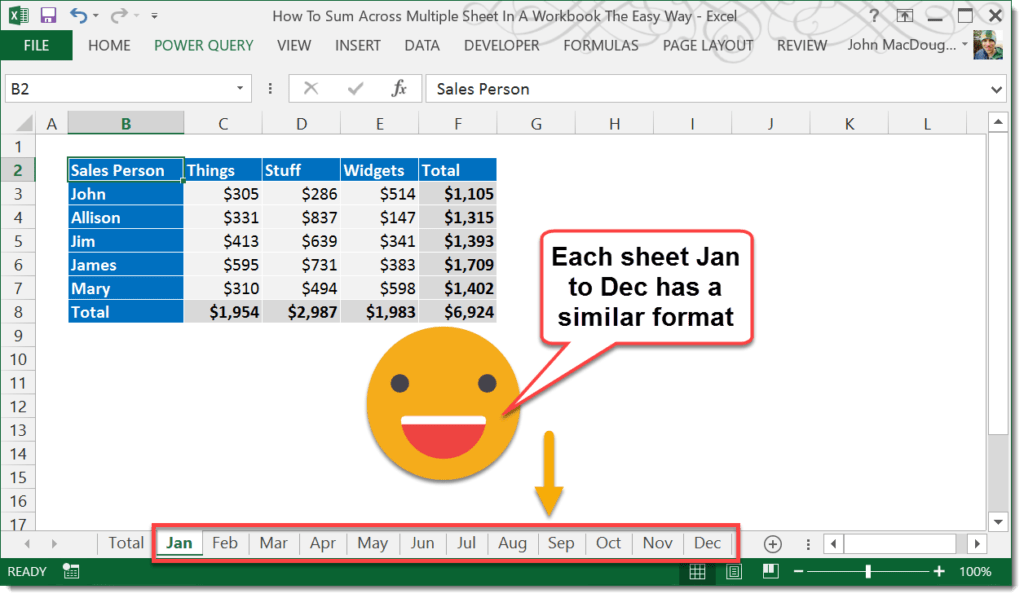
In this example, you have a table of sales figures each in a separate tab named Jan through Dec.
Each sheet is the same format with the table in the same position within each sheet.

=Jan!C3+Feb!C3+Mar!C3+Apr!C3+May!C3+Jun!C3+Jul!C3+Aug!C3+Sep!C3+Oct!C3+Nov!C3+Dec!C3If you wanted to create a Total sheet and have a table in it that sums up each of the tables in the Jan to Dec sheets, then you could use the above formula and copy it across the whole table.
Creating this formula isn’t very efficient though, as it requires selecting the Jan sheet, then selecting the cell C3, then typing a +, then selecting the Feb sheet, etc.s
Going through 12 sheets in all. There is a better way!

Add the sum formula into the total table.
- Type out the start of your sum formula
=SUM(. - Left click on the Jan sheet with the mouse.
- Hold Shift key and left click on the Dec sheet. Now select the cell C3 in the Dec sheet. Add a closing bracket to the formula and press Enter.
Your sum formula should now look like this =SUM(Jan:Dec!C3).

The formula will sum up C3 across each of the sheets from Jan to Dec.
You can also use this technique with other formulas like COUNT, AVERAGE, etc. An easier way over cycling through each sheet individually.
 👉 Find out more about our Advanced Formulas course!


This is also referred to as 3D formulas. Tiling worksheets or workbooks side by side is the quickest and less confusing method to use when doing this.
Doesn’t work if you have any spaces or numbers in your sheet names. To fix, rename the sheets using only alphabetics and no spaces or put a single quote before the first sheet name and a single quote after the second sheet name before the exclamation mark.
Thanks for the tips!
Thanks for having this available! I’m very inexperienced with excel and you made what I needed to do easy to understand.