This is a guest post by Alan Murray from Computergaga.
Data Validation is a very useful Excel tool. It often goes unnoticed as Excel users are eager to learn the highs of PivotTables, charts and formulas.
It controls what can be input into a cell, to ensure its accuracy and consistency. A very important job when working with data.
In this blog post we will explore 11 useful examples of what Data validation can do.
To apply these Data Validation rules;
- First select the range of cells you want to apply the validation to.
- Click the Data tab and then the Data Validation button on the Ribbon.
- In the Settings tab, select the validation rule criteria.
Allow Uppercase Entries Only
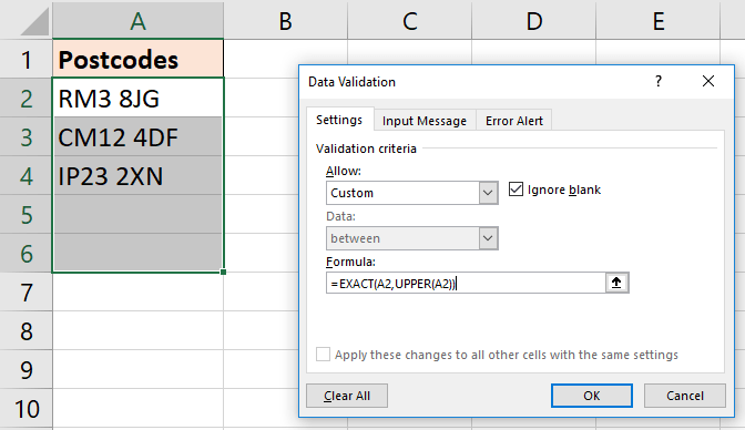
You may need to ensure that data is entered in uppercase, such as this example of UK postcodes being entered.
The cells need to accept the entry of both text and numbers, but the text must be uppercase.
For this we can use a formula with the UPPER and the EXACT functions.
The UPPER function probably speaks for itself. It converts text into uppercase.
The EXACT function is used to compare the cell entry with the uppercase version to see if they are the same. If they are, then the entry is valid.
For this example, the validation was applied to range A2:A6. Select Custom from the Allow list and enter the following formula into the Formula box.
Prevent Future Dates
Entering dates is very common on a spreadsheet. Unfortunately users entering the wrong date is also commonplace.
By using validation rules, we can limit the mistake a user may make.
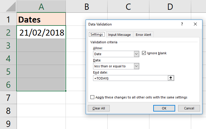
In this example, we prevent the entry of a future date. Maybe users are recording a transaction that has occurred. Therefore, it must be a date in the past or todays date.
Select Date from the Allow list and then Less than or equal to from Data.
In the End Date box, type the formula below.
The TODAY function returns the current date from the computer. Incredibly useful. Check out more great Excel date functions (https://www.howtoexcel.org/category/functions/date-and-time/).
Creating Drop Down Lists
Creating drop down lists is the reason most people become familiar with the Data Validation feature. Creating lists is a simple and effective way of controlling data entry.
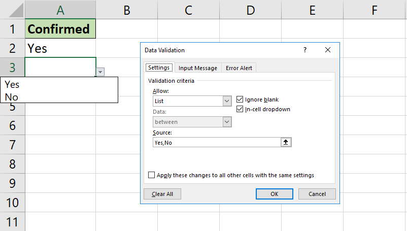
Select List from the Allow list. You can then either type the list items directly into the Source box separated by a comma, or refer to a range of cells that contain the list items.
When you need a simple list such as Open and Closed, or Yes and No, then typing the entries in makes sense.
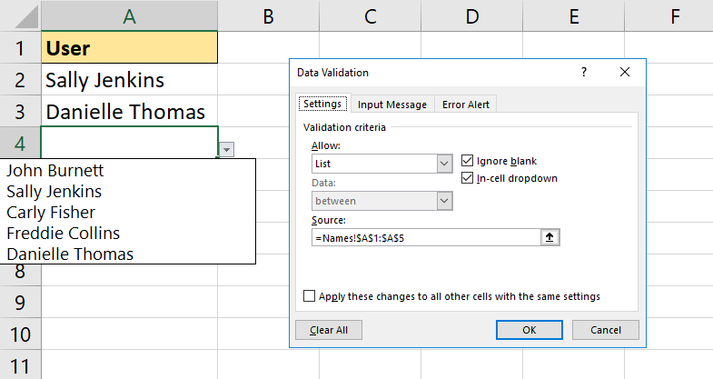
When you need a more dynamic list for items that change over time such as lists of products, places and people, then referring to a range makes sense.
For this list, click in the Source box and then go and select the cells that contain the items.
In this example, the items were in range A1:A5 of a sheet called Names.
Dependent Drop Down Lists
Let’s take our drop down lists further and create dependent lists. For these lists, the item selected in one list will affect what options appear in the next list.
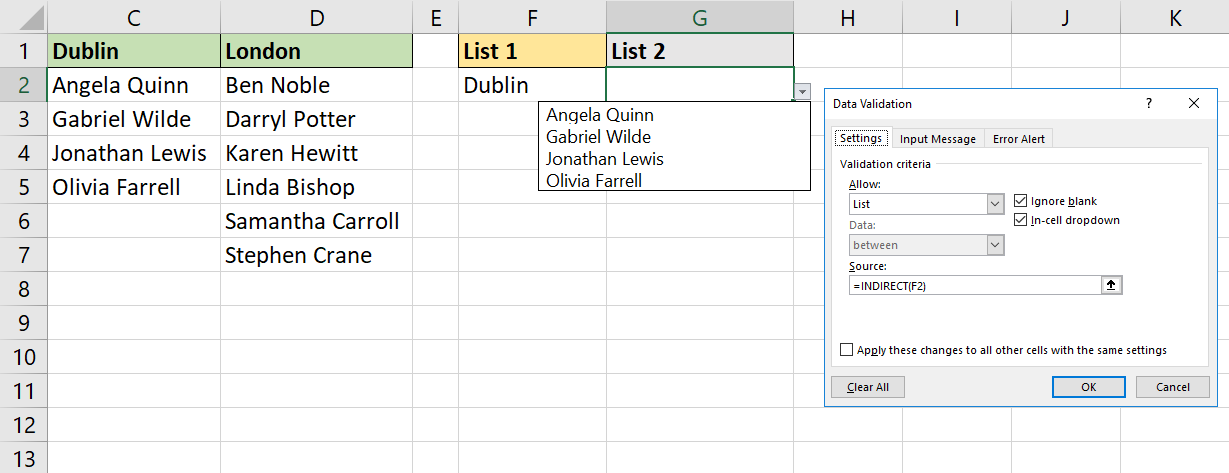
In the example below, we have a list of cities in cell F2. The selection from this list affects what names appear in the next list in cell G2.
To achieve this, we first must name each list. For example, range A2:A4 is named city, range B2:B6 is named cardiff and so on.
Follow these steps to create a named range.
- Select the range to name e.g. A2:A4.
- Click in the Name Box to the left of the Formula bar.
- Type the name you would like to apply and press Enter.
The list in cell F2 is created just like in the previous example. In the Source box you can type =city to reference the named range.
For the dependent list in cell G2, the selection in cell F2 needs to be converted into a reference to the named ranges. This is done using the INDIRECT function (Learn more awesome examples of the INDIRECT function).
A common issue when creating dependent lists is the use of illegitimate characters in named ranges. You cannot begin named ranges with a number, or use spaces and some other symbols.
So, if items in your list use spaces, or start with numbers it presents an obstacle. Learn how you can overcome this issue in the video below.
Prevent Duplicate Values
Duplicate values are a very common problem in Excel. There are many techniques for identifying and removing duplicates, but it would be better if you could prevent them in the first place.
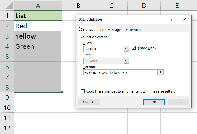
By using the COUNTIF function in a custom formula we can.
The formula below counts the occurrences of the inputted value in the range A2:A8. If the answer is 0 then the value is unique and allowed.
Allow only Numeric or Text Entries
The ISNUMBER function can be used to create a validation rule that only allows the entry of numeric values in a cell.
Select Custom from the Allow list and use the formula below. In this example, cell A2 is the upper left cell of the selected range of cells.
This will allow any numeric values only including dates and times.
To allow text values only we could use the ISTEXT function in the same way.
Validate an Entry Based on Another Cell
You can create Data Validation rules that are based on the value from another cell by writing a custom formula.
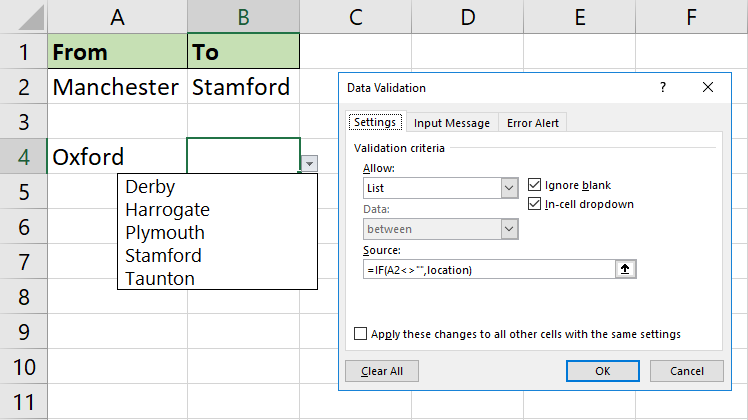
For example, maybe you only want a drop down list to appear if another cell is not empty.
The following IF function will test if cell A2 is not empty, and if so show the list from the location named range.
Allow the Entry of Weekdays Only
When entering dates, you may need to restrict a user to the entry of specific days of the week. We can achieve this with the WEEKDAY function.
For this example, we shall restrict entry of dates that are Monday to Friday only. The formula below can be used for this.
The WEEKDAY function returns a number that represents the day of the week. In the WEEKDAY function, the 2 specifies that a week starts on Monday as 1 through to the Sunday as 7.
In this validation rule, the returned value must be less than or equal to 5. This excludes Saturdays and Sundays.
Restrict the Text Length
Entries may need to be of a specific text length, or no more than a certain number of characters. Creating a validation rule can help us ensure this.
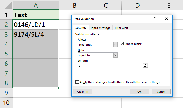
In this example, I want to confine the text length to exactly 9 characters.
Select Text length from the Allow list, equal to from the Data list and then type 9 for the length.
Entries Contain Specific Text
Using Formulas in validation rules enables us to test and validate for almost anything.
In this last example, we ensure entries contain specific text.
The FIND function is used to search for a specific string of text (“ENG” in this example) and return its position within the cell. If FIND does not locate the text, an error is returned.
The ISNUMBER function is used to check if the FIND function was successful (if it returned a number). If it did, then ISNUMBER returns True, otherwise it returns False. This completes our validation test.
Here is the formula to use.
Note: The FIND function is case sensitive. The SEARCH function can be used instead if you do not need to match the case of the text.
Create Meaningful Error Messages
We have looked at 10 Data Validation examples in this article. However, if a data entry mistake is made the same validation is shown, regardless of the validation criteria.
The great news is that you can create your own error messages to effectively communicate what may have gone wrong to the user.
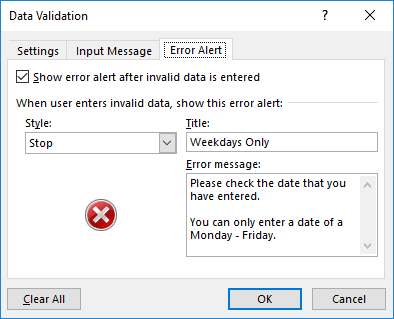
Click the Error Alert tab of the Data validation window.
Select a Style from the list of Stop, Warning, or Information.
- Stop will prevent invalid data from being entered.
- Warning displays the error, but with the choice to allow the entry or prevent it.
- Information display the error, but does not prevent the data entry at all.
Type a Title and Error Message for the error alert.
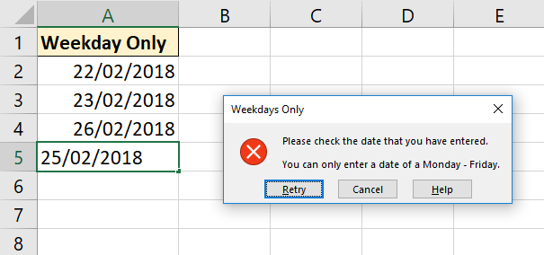
Let’s take the example of allowing only the entry of weekdays into a cell. You could create an error message like this.
Conclusion
I believe Data Validation is an undervalued tool of Excel. Without clean data our PivotTables, charts and formulas will not function correctly.
This feature provides a method of limiting mistakes and collecting clean data on entry.
Data Validation cannot help though when receiving data from other databases, workbooks and websites.
If this is something that you do, I heavily encourage you to check out the Power Query feature of Excel. A powerful tool for establishing connections and automating the process of cleaning and transforming data from external sources.
About the Author
Alan is the founder of Computergaga and has a large YouTube following where he shares Excel tips and tutorials. He lives in the UK with his wife and 2 children. His passions for Excel and data keep him busy, but when he has free time he enjoys running and hiking.






 👉 Find out more about our Advanced Formulas course!


Nice Compilation Alan………..Thanks for sharing.
Wonderful Job Sir,
How do I enter Data Validation so that a new row iterates to the next row reference? For example so that a Data Validation setting in Cell C38 that references Cell C39 on line 39? For some cells its works and for others it doesn’t increment in the Data Validation Settings/Source field.
Hi :
How do we disallow entry in dropdown cell and only allow the selection of list item in excel?
I don’t believe this is possible. Potentially with some VBA. But even if they type, it will get validated.
“How do we disallow entry in dropdown cell…?”
On the Error Alert tab in the Data Validation window, select the “Stop” Style and add a message that explains what the user must do instead.
Oh, and choose List in the Validation criteria > Allow field.
Data validation is such a cool feature so im always intrin seeing the different ways people can use them.
Absolutely. And so often overlooked to learn sexier tools like PivotTables and charts. But without good data, its over.
Thank you so much for the information = Very Helpful!
How can you set up a Data Validation that will allow specific text but will not allow you to enter a space before or after that text?
i.e. they can only enter EXE, PRO, SPEC in the cell – but not EXE , SPEC , PRO.
Thank you for your help! It is greatly appreciated!!!
You can use the list option for this. Either enter those words separated by a comma, or refer to a range of cells where they are written.
If you don’t want the list you can uncheck the in-cell dropdown box.
Use this formula in custom option of data validation
=ISERR(FIND(” “,E4))
use TRIM() in the validation formula:
=TRIM(cellref)=cellref
Thank you! But I don’t like to use drop down list because they show up so small. I do put the specific words that can be entered… But I’d someone accidently puts a space behind the letters then my formulas in other areas will not pick up the cell information that has a space in it. 😭😭😭😭
Yes, just uncheck the in-cell dropdown and you will not get a list. You can use a formula such as this – A1=TRIM(A1) to prevent spaces before and after. This assumes your selection starts at A1. We then just need it to restrict it to your three words also.
Your other formulas could include the TRIM() function so that even if spaces are wrongly added, those formulas would reas them correctly.
Thank you.
I’m not sure I’m explaining my self correctly.
Can you have multiple Data Validations on the same cells?
So let’s just say… I have selected cells A1..D20
I have done a Data Validations that only LTR, STR, EXE, PRO can be entered in these cells. Which works.
So how can I do a data validation with a TRIM in these same cells A1..D20 so that if they enter a Space behind these letters it will not let them?
If you make a list in Data Validation by referring to a range of cells, and not typing them into the source box. This will also prevent the trailing space scenario. I just wrote your 4 items in cells A1:A4 on a sheet. Named the range items. And then used =items in the source of a Data Validation list.
Remember you can turn of the in-cell drop down. You don’t have to have the list. Just this option for your four entrants.
Thank you! THANK YOU! THANK YOU!!!!
That takes care of the trailing space… . Now can I am them be entered in with ALL CAPS?
The EXACT function can be used to ensure that text matches case, but I am not sure this can be used with the list functionality. I think this may be too much for Data Validation.
Did you ever get the answer you needed to this question?
HI,
I need to use a list of products codes and in a specific cell to return the product code that’s matching that code once I start entering.
What can I use? Data validation with a formula..to Search and Find the product code and show it once I start typing? Or something else?
I need to limit the typing(entering the codes) to a list (range) and display the code once I start typing.
Thanks
Displaying a list whilst typing is not something that Data Validation does as standard. There are tutorials on the web of people using VBA or complex formulas to get an imitation going. A lot of effort for little reward and will also increase Excel’s processing. Hopefully a future version will bring this.
Hello,
Thanks for the reply.
Another project I am working on, requires me to use a workbook with 3 different columns that can be filtered(with regular filter) and then get final results in the 3 rd column. This is to reduce the drop down list to a narrow one.
In the actual workbook I need to show that final result in a drop down menu.
I am thinking of a searchable table with results to be displayed.
Is there any way I can do that using simple functions in Excel?
An example would be very helpful.
Thank you!
Hi Lyl,
It sounds like you would like dependent drop down lists. I have a video on setting these up here – https://youtu.be/5nb84p2wX-c
Hello
Thank you so much for the information and for sharing your knowledge!
Let’s say I have to create two drop-down menus with one specifying the Start date and another the End date – my dates are listed on my active sheet (eg. 12/31/2014, 12/31/2015 etc.)
How can I make sure the End date is always greater than or equal to Start date?
Thank you!!!
Hello,
Thank you so much for the information and for sharing your knowledge!!
Question:
Let’s say I had to create two drop-down menus: one specifying a Start date and the other an End date, with the dates listed on my active sheet (eg. 12/31/2015, 12/31/2016 etc.) How can I make sure the End date is always greater than or equal to the End date?
Many thanks!
A cell can only contain one validation rule if you are using it for a drop down. You could lose the drop down and use the Data Validation for the greater than rule instead.
Or if you want to keep the dropdown, maybe use a different technique such as Conditional Formatting. Instead of stopping the user, you could get the cell to change colour if it is greater than or equal to the start date.
In Conditional Formatting, if the start date is in A2 and the end date in B2 then the formula could be =B2<A2
I HAVE A PROBLEM THAT I HAVE TWO DIFFERENT TYPES OF DATA.
I WANT THAT WHEN ONE TYPE OF DATA APPEARED BY VALIDATION THEN ITS TOTAL SHOULD BE PLACED IN A CELL
AND WHEN I CHANGE THE DATA OF SAME CELL BY VALIDATION BY CHOOSING 2ND TYPE OF DATA THEN ITS TOTAL SHOULD BE PLACED IN ANOTHER CELL , NOT PREVIOUS.
Hi Yashraj, a cell can only contain one format type – number or text. Maybe you don’t want validation in the cell. Either way you can control what cell the total is shown in by using formulas in those cells. Depending on your scenario a simple IF may suffice to test the validation cell and run the formula or not.
I found “Validate An Entry Based On Another Cell” particularly useful, Alan, and immediately applied it to a current project using Table names in this formula:
=IF(ISNUMBER(E6),INDIRECT(“Table_Title_OBJECT_TYPE[System ID]”),INDIRECT(“Table_Title_OBJECT_TYPE[Hierarchy]”)).
This allows users to pick from a list (Hierarchy) or to enter the Hierarchy’s ID number if they know it already.
Here’s a variation using Named Ranges:
=IF(G2=”HH”,HH,IF(G2=”NS”,NS,IF(G2=”Bot”,Bot)))
Thanks for the tip!
You’re welcome Philip. Thank you.
Hi,
Lets say I hard code 1,0 while creating a drop down, and change the format to display the result as YES or NO. How do I apply this format to the drop down list as well, and not just the result?
The drop down list content cannot be formatted, just the result of that content by formatting the cell that the drop down is in.
Its Awesome – Very well explained – I managed to clear lot of doubts – Thank you
You’re very welcome Asoka. Happy to help.
Hello,
In your “Prevent Duplicates” section, for a value to be unique, the COUNTIF formula must return 1, not zero. That’s how it works in my Excel. If I put zero, any entry is refused.
Quite right Patrick. I’ll get it changed.
is there a way I can enter only specific 2 to 3 words and dates in a cell, eg if an activity is completed then date of completion, if activity is pending than “Pending” if issue “Issue” apart from these any entry should not be possible
Sure Varaprasad. The three options would be your classic drop down list. For the date of completion, you could make this cell dependent upon completion being entered in another cell if you wanted. An example of a rule based on another cells value is shown in the tutorial.
Hi Alan,
Is there a way to combine a drop down list together with another validation such as Prevent duplicate values?
No sorry, not within the Data Validation rules. You would have to look at using a macro for this validation check on top of the drop down list one.
Thanks Alan.
I have a little complex problem.
I have two tables T1 and T2, and both have common columns say “Name” and “City”. Now, how to add a data validation list to T2.Name that is filtered with T1.Name where T2.City = T1.City.
Basically I want to filter the Names drop down in the T2.Name only with the T1.Names from the same City.
Thanks in advance.
My pleasure. This sounds like a lookup formula instead of a Data Validation list. If it is filtered by T1 for one city, you wouldn’t need a list.
VLOOKUP will do the job.
Good to see the reply Alan.
Certainly I need a data validation drop down list, just that it has to be filtered based on the current table’s City (common column between 2 tables) value in the lookup table.
So for T2 Name column dropdown to be filtered and show only those Names who live in that city.
To up the complexity a little bit😀 this filtered, relevant list should be ‘distinct’ Names
Oh ok. Are you using 365 because if you are, with the new UNIQUE and FILTER functions this task is easy.
If not, PivotTables could be used to create the unique city lists and dependent drop downs can be created from them.
how to put the validation for Mandatory columns does anyone know..
You are probably better off doing this in VBA. Data Validation will only work when someone attempts entry to a cell. VBA could be used to check cell values (ensure they have been used) prior to submitting, saving, printing or whatever the action may be.
Hi Alan.
Thanks for this nice post.
I have specific query. I have used data validation input message option to add comments to some specific cell in excel.
However, there is no indication that the particular cell has some message. Its only when I click on the cell, I get to see the message.
In the case when we add a comment for a cell, there is a small red arrow in the cell corner which indicates that a comment is entered for the cell. Is there some similar kind of arrangement that we can do for data validation message.
Thanks
–Ashutosh
Hi Ashutosh, there is not a setting for this in Data Validation. Sorry.
Hi Alan, Is there a way to create a drop down list that contains a data name and other text values? For instance, want a drop down list of Year(Today()) – 1, Year(Today()), None, Both. Thank you!
Not sure exactly what you mean Cal. But looking at your example, I would put those formula into a cell somewhere along with the text values. And select them for the DV list.
Hi can someone help with a formula in excel that ensures that cell can only be 9 characters long. And the following must show if the entry does not meet the requirements: a stop symbol and an error message that says: the text lenght must be 9 characters
Hi Elizna, this is shown in the tutorial. There is an example for “Restrict the Text Length” and then one for “Create Meaninging Error Messages”.