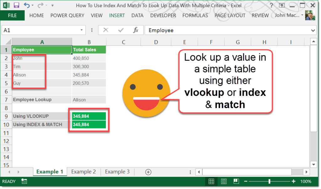
Looking up a value based on one criteria
Let’s say we have a table with employees and their total sales and we want a formula to return the total sales based on the employee.
Now, if we want to get Allison’s sales, we could use a VLOOKUP formula using this formula.
=VLOOKUP(B7,A2:B5,2,FALSE)
Or, we could get fancy and use an index match combination using this formula.
=INDEX(B2:B5,MATCH(B7,A2:A5,0))
Looking up a value with a row criteria and a column criteria
Now suppose we have a similar table and the employees sales are split out between sales in the East and sales in the West. Now let’s say we need to lookup Guy’s sales for the West.
=INDEX(B2:C5,MATCH(C7,A2:A5,0),MATCH(C8,B1:C1,0))
Looking up a value with two or more row criteria
Ok, what happens now if we have the same data but it’s not laid out in a two dimensional range like above (ie one lookup value going down the rows and one lookup value going across the columns)? Let’s say we have a column with the region and we’re still tasked with finding Guy’s sales for the West.
=INDEX(C2:C9,MATCH(C11&C12,A2:A9&B2:B9,0))
In this case we can concatenate our lookup values and lookup ranges to use an array formula.
Enter formula with Ctrl + Shift + Enter
When you enter this formula, instead of pressing enter in the usual way, you will need to press Ctrl + Shift + Enter. If you’ve done this correctly, then you should see a set of { } curly parenthesis around the formula in the formula bar.
If we have 3rd, 4th etc… criteria in additional columns, we can use this same array function approach to lookup values.


 👉 Find out more about our Advanced Formulas course!


I am trying to use INDEX and MATCH with multiple criteria and I keep getting a formula error message. In the “result” cell, I want to have the formula reference my set of data (located on another sheet), then match to a value in the row above (in the same column as the “result” cell) as well as match to a value in the column to the left (on the same row as the “result” cell) and return the “result” value. So two criteria are being reference and as you copy the formula across the sheet, the “row above” reference changes because you are in a new column, but the “column to the left” reference stays the same. And vice versa as you copy the formula down the sheet. How do I do this with INDEX and MATCH?
Sounds like an issue with setting the correct absolute or relative range reference. Try highlighting the various ranges and press F4 to cycle through the different referencing. Try them out until you get something that’s working correctly, unfortunately I can’t see what the issue is to help out any more.
Thanks John. I was able to figure it out as I changed my MATCH lookup ranges to be a “vertical” lookup first, followed by a “horizontal” lookup. This worked and I’m good to go. Thanks for your input.
Good to hear!
I am attempting to use INDEX-MATCH with multiple criteria; but I’m running into an issue when I copy the formula to the next column. It seems to have something to do with the brackets, but I cannot figure it out…when I try to copy the formula down, I get an error message that says “You can’t change part of an array.”
I’m new to using INDEX-MATCH, so I’m just totally confused.
Thanks for your help.
I think you may be trying to paste over the copied cell. Try copying the cell, then moving the range off that cell and then pasting.