Do you want to know how to add arrows in Excel? Here is how you can do that in simple steps.
MS Excel isn’t just software for calculation and data storage. It can also be used for graphical representation, annotation, and presentations. You can create a variety of charts and graphs utilizing its data with the help of this software.
If you’re using it to visually compare two datasets, you may need to add arrows in it. Also, arrows are a great way to indicate data flow and process flow that the audience can comprehend without any difficulty.
So the good news is, that you can add arrows in Excel using multiple methods. But the question is, what are those methods? Also, you need to know the exact steps to implement those methods to avoid confusion and save valuable time.
Therefore, I bring you the proven methods to add arrows in Excel. You can choose from these methods as your choice and include arrows in suitable places in the spreadsheet data.
What Is an Arrow in Excel?
Arrows are concise graphical elements representing actions, progression, or navigation in Excel. It can also act as a symbol to show a connection between two or more cells visually. In Excel, you can use arrows in cells, charts, Conditional Formatting, text boxes, shapes, and so on.
Reasons to Add Arrows in Excel
- During the illustration of the direction of information or process, you need to use arrows to indicate the flow of data or the sequence of a process.
- In a chart or graph, arrows are used to highlight trends or patterns in your data, such as indicating a significant increase or decrease in a data series.
- In interactive or instructional spreadsheets, arrows are used to guide users through specific steps or instructions for them to follow.
- When you use Excel data for analysis, you can use arrows to show the relationships or correlations between variables. Thus, it becomes easier to interpret the results of your analysis.
- When comparing multiple datasets, arrows can be used to visually represent higher, lower, or equal values so that the audience can make quick comparisons.
- While making reports or presentations, you need to add arrows to draw attention to important trends or specific cells.
- Finally, arrows can enhance the visual appeal of your spreadsheet so that it looks more engaging and understandable. Including arrows will help you create a clear visual hierarchy.
Now that you’ve gathered a basic idea of Excel arrows, find below the methods to add these in Excel:
Add Arrows in Excel Using Shapes in Excel
The Shapes tool of Excel consists of vector art for Lines, Rectangles, Basic Shapes, etc. You’ll find arrow shapes under the Lines and Block Arrows section.

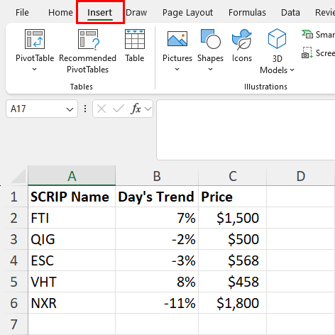
To insert an arrow from the Shape tool, go to your dataset or worksheet in Excel. Then, click the Insert button on the ribbon menu.

Find the Illustrations block and click on the Shapes button. Now, choose any arrow you like from the Lines and Block Arrows section.

The Excel cursor will change into a black crosshair. You can either draw the arrow on the cell or click to get the default arrow. Drawing an arrow allows you to customize the size of the arrow shape compared to the large version of the default shape.

You can now copy-paste the arrow on other cells in your dataset. This arrow is suitable when you need to create a few arrows but not for the whole dataset.
Insert Arrows in Excel Using SmartArt in Excel
SmartArt arrows are suitable for creating process flows in Excel. The SmartArt library contains pre-designed grouped arrows. After inserting one such graphic, you just need to edit the text of the shapes. You’ll find many such arrows in the Process and Relationship category of the SmartArt library.

To get a SmartArt graphic arrow on Excel, go to the Insert tab. Click the SmartArt button inside the Illustrations block.
On the Choose a SmartArt Graphic dialog, select either Process or Relationship category.

Suppose, you’ve chosen the Relationship SmartArt category. On the right side menu, click on a SmartArt graphic like Diverging Arrows. Click OK to insert the vector graphic into your Excel worksheet.

The arrows come with a left-side text navigation panel. There, you can click [Text] placeholder text and enter your content. Click on any blank cell on the worksheet to enter the SmartArt graphics.
📒Read More: how to create an organizational chart in Excel!
Add Arrows in Excel Using Icons
The latest Excel for Microsoft 365 desktop app comes with the Stock Images library. You can access the library from Insert > Illustrations > Icons menu. However, you can only access these premium icons or stock images if you’ve got a Microsoft 365 subscription.

If you know you’ve got access to Icons in your Excel app, go to the worksheet where you want to add arrows. Now, go to Insert and click on the Icons button. The Stock Images dialog will pop up. It may take a while to load content from Microsoft 365 server.

Click on the Search field and type “Arrows.” Hit Enter to list all the arrows in the Stock Images dialog box.

You can now choose one or many arrows from this library. Click the Insert button to add the arrows to your Excel worksheet.

Excel will download the icons and hence it may take a while. The added arrows are in large thumbnail sizes.

Click on an arrow and use the orientation handle to adjust the orientation of the arrow.

Now, click on the Place in Cell button to add the arrow to a blank cell automatically.
Insert Arrows in Excel Using 3D Models in Excel
If you want to enhance the visual attraction of your Excel worksheet, you can use 3D arrows. You can find many 3D arrows in Insert > Illustrations > 3D Models.

Go to your dataset where you want to add 3D arrows. Click the 3D Models drop-down list on the Insert tab and click on the Stock 3D Models option.

The Online 3D Models dialog will show up. Type “Arrow” into the Search panel and hit Enter.

Select an arrow you like and click the Insert button to insert the 3D graphics into your worksheet.

Use the 3D orientation handle in the middle of the graphics to adjust the orientation.

Now, resize the graphic using any of the shape outline points.

Place the arrow on a cell where you want that. You can copy and paste it onto other cells.
Add Arrows in Excel Using Symbol Tool
The arrows that you add to your worksheet from the Symbol tool are suitable for programmatic use in Excel formulas.

Suppose, you need to insert up and down arrows in column C depending on values in column B.

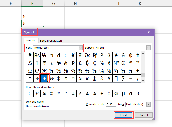
Highlight the F2 cell and insert the up arrow from Insert > Symbols > Symbol > Font (normal text) > Upwards Arrow.

Now, select the F3 cell and insert the Downwards Arrow.

Now, go to C2, enter the following formula, and hit Enter:
=IF(B2>0,$F$2,$F$3)
Now use the fill handle to copy and paste the formula to other cells in column C.
Using Windows Emoji Tool
You can also quickly use the Windows Emoji app to add arrows to your Excel worksheet.

Go to the target worksheet and select a cell where you want an arrow symbol.

Press the Windows + Period keys to launch the Windows Emoji app.

Click on the Symbols emoji tab and choose an arrow from the list of emojis. Click on it to enter the arrow into the cell and close the Emoji app.

Now, repeat the above steps to add a downward arrow.

You can now copy and paste these arrows wherever you want in the spreadsheet.
Add Arrows to Charts in Excel
If you need to add arrows in data series or columns in Excel charts, here’s how you can do that:
Insert Arrows Into a Line Chart

Go to the Excel worksheet containing a chart and click on the Data Series. Right-click and select the Format Data Series option on the context menu that appears.

On the Format Data Series navigation pane, click on the Fill & Line tab.

If you need an arrow at the end of the data line, click the End Arrow Type drop-down and choose the arrow style you want.

You should see an arrow on the data line in your line chart.
Add Arrows to a Column Chart
Unfortunately, the End Arrow Type feature doesn’t work when you try to format the data series of a column chart.

Therefore, you must use the arrows from the Block Arrows category in the Shapes library of Illustrations command block in the Insert tab.
Add an Arrow:Up shape from the Shapes library and resize it to fit the top of the columns or bars of the chart.

Click on the shape again and go to the Shape Format tab. There, click the Shape Outline drop-down and choose No Outline.

Now, copy and paste the arrow shape on other columns in the chart.
Add Arrows in Excel Using Conditional Formatting
If you want to insert colored arrows that indicate the increase or decrease of values in cells you can use the Conditional Formatting tool in Excel.

Go to your worksheet and highlight the dataset where you want to insert arrows. Then, click the Conditional Formatting drop-down in the Styles block of the Home tab.

Hover the cursor over the Highlight Cells Rules option and click on the More Rules option in the overflow menu.

On the New Formatting Rule dialog choose the Format all cells based on their values option and change Format Style to Icon Sets.

Click on the Icon Style drop-down and choose the 3 Arrows (Colored) option. Also, click on the yellow arrow and change it to a red arrow.

Enter the Conditional Formatting logic under the Value fields. To change the type of values click on the Type drop-down list.

Click OK to apply the formatting rule and you should see green arrows for positive percentage and red arrows for negative percentage values.
Insert Arrows in Excel Using Excel VBA
The best way to add in-cell arrow symbols in a large dataset in Excel is VBA scripting. Excel VBA scripting can go through the reference cell ranges to figure out if the values are positive or negative.
Excel shall insert up arrows for cells with positive values and down arrows for cells with negative values.
Find below the script you can use:

Sub InsertArrowsToLeft()
    Dim ws As Worksheet
    Dim cell As Range

    ' Set the worksheet
    Set ws = ThisWorkbook.Sheets("Sheet3") ' Change "Sheet3" to the name of your sheet

    ' Set the range to B2:B6
    Set Rng = ws.Range("B2:B6")

    ' Loop through each cell in the range
    For Each cell In Rng
        ' Check if the cell value is positive, negative, or zero
        If cell.Value > 0 Then
            ' Insert up arrow for positive percentage to the left
            cell.Value = ChrW(&H2191) & "  " & cell.Value
        ElseIf cell.Value < 0 Then
            ' Insert down arrow for negative percentage to the left
            cell.Value = ChrW(&H2193) & "  " & cell.Value
        End If
    Next cell
End Sub
To customize this VBA script, follow these instructions:
- Change
"Sheet3"to the actual worksheet name where you’re working. - Replace
"B2:B6"with the cell range where you want to insert up and down arrows.
If you’re wondering how to utilize the above VBA script, read this article on How To Use The VBA Code You Find Online.
Conclusions
As an Excel user, you must know that the application can be used for data visualization and reporting. While using it for this purpose, you may need to use arrows to indicate data flow direction or improve the visual appeal of your spreadsheet data.
For this reason, it’s essential to know how to add arrows in Excel. In this article, I’ve included several approaches to add arrows. Depending on your expertise level, you’ll find some methods to be easy and others to be comparatively complex.
So, it’s better to try these techniques one after another and see which one you can perform easily. When you’re done, don’t forget to share your experience of implementing these approaches. If you know any other methods of adding arrows that are not mentioned here, mention that in the comment section.
 👉 Find out more about our Advanced Formulas course!


0 Comments