When you know how to combine two columns in Excel you can better manage the raw dataset to create meaningful data models for complex data analytics and visualizations.
Often, business apps or website servers may collect and segregate data in columns incorrectly. These data sources may get confused with column headers like full names, timestamps, product codes separated with text and numbers, phone numbers with country codes, survey responses, and more.
Hence, you find these inseparable data points in different columns instead of the same column. The skill of combining columns in Excel helps you to tackle such challenging situations.
In this tutorial, I’ll walk you through step-by-step instructions, providing insights and techniques to streamline your data management process of separate columns. Whether you’re a seasoned Excel user or a beginner seeking to enhance your spreadsheet proficiency, you must learn this column merging tactic in Excel.
Why Would You Want To Combine Two Columns in Excel?
The primary need to combine two columns in Excel is to create columns of meaningful datasets. You could find an Excel dataset where the first names, last names, phone numbers, country codes, etc., are separated in an array of many other columns.
By learning the process of combining columns in Excel, you can bring related columns side by side and merge related datasets into single columns.
Find below other prominent reasons to combine two columns in your worksheet:
- Combining columns declutters data presentation. Your audience can easily concentrate when you present datasets or Excel tables.
- By merging them, you can get a holistic view of the dataset when you reduce the number of columns. Therefore, you can find patterns in the raw data.
- A unified column allows for quicker sorting and filtering of data based on specific criteria.
- Combining columns reduces the chance of errors during data entry by consolidating related information.
- Merged columns provide a clear basis for creating charts and graphs, thus aiding visual representation.
- Combined columns enable smoother utilization of VLOOKUP and INDEX – MATCH functions for data retrieval.
Use Flash Fill
Flash Fill allows Excel to recognize patterns from your actions and repeat the same task. You can show a data entry pattern to Excel using your dataset. Then, using the Flash Fill command, you can make Excel perform those tasks in a single click.

Open your Excel spreadsheet and navigate to the worksheet containing the columns you want to combine.
Click on the cell in which you want to start the combined column data. Type in the desired format for the combined information.
For example, in the above screenshot, I combined first and last names separated by a space by typing the format in the first cell.

Now, move to the Data tab on the Excel ribbon. Locate and click on the Flash Fill option in the Data Tools group.
Alternatively, you can use the keyboard shortcut Ctrl + E on a Windows PC and Command + E on a Mac.

Excel will automatically detect the pattern based on the first cell you edited and apply the same format to the entire column.
You can review the combined data to ensure it meets your expectations. If needed, you can manually adjust specific cells.
Use the Equals and Ampersand
If you’re using a dated Excel software like Excel 2010, you won’t find the Flash Fill option. Instead, you can use a combination formula involving the equals sign and the ampersand symbol.
Suppose, you want to join the data of columns A and B in column C. Here’s how you can use this combination formula:

- Highlight C2.
- Copy and paste the following formula in C2:
=A2&" "&B2
- Hit Enter to apply the formula.
- Excel will combine the data of the first two cells of the source columns.
- Use the fill handle to apply the formula across the column.

Copy the combined content, press Ctrl + Alt + V, and choose Values in the Paste Special dialog to convert formula arrays in the cells to text values.
Use the CONCAT Function
If you’re using Excel 2016 or newer software on your PC or Mac, you can use a more straightforward formula to combine two columns in Excel. This is the CONCAT function.
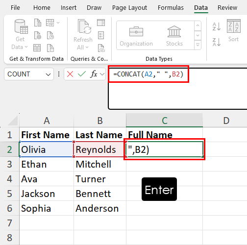
Access your Excel spreadsheet and go to the cell where you want to display the combined data. Suppose, it’s C2 and you’re combining names in columns A and B.

In the highlighted cell, enter the following formula and hit Enter. Excel should automatically join the first two cells of the target columns.
=CONCAT(A2," ",B2)
Now, you can either copy and paste the above formula across column C. Alternatively, you can drag the fill handle down column C until the last non-blank row in the adjacent columns A and B.
Use the TEXTJOIN Function
Sometimes, there could be empty cells in one of the two rows you’re set to combine in Excel. To instruct Excel to ignore those empty cells, you can use the TEXTJOIN formula.

Here’s the formula you need to use in any cell of your choice:
=TEXTJOIN(" ",TRUE,A2,B2)Here’s how to modify the formula:
A2is the reference for the second cell in the first column to be combined- Similarly,
B2is the cell address for the second cell in the second column " "is the delimiter I’m using in this example. This is a space to give the output as Olivia Reynolds. You can use any delimiter symbol like comma, semicolon, @, etc. Double quotes around the delimiter are mandatory though.
This is a fairly new formula in Excel and available since Excel 2019 for Windows, Excel 2019 for Mac, and Excel for the web app.
So, you could face backward compatibility issues when sharing the workbook with a person using an Excel desktop software older than Excel 2019.
Use the Notepad App on a Windows PC
Often, data extracted from software or servers contains unwanted characters in the columns. If you use any of the above methods, you risk including those unnecessary characters in your final Excel dataset after merging two columns.
Here comes Notepad. It’s a simple text editor and the best tool to get rid of funny symbols from columns before merging.

Go to your Excel workbook and copy the two columns that need merging.

Open a new Notepad file and paste the content there.
Press Ctrl + H to launch the Find & Replace tool of Notepad on a Windows PC.

In the Find what field enter the characters you want to weed out. For example a Right Tab or simply Tab.
In the Replace with field enter the replacement for the symbols you’re eliminating. For example, a space.
Hit the Replace All button.

Now, copy the Notepad file content and paste it on a column where you want to combine two columns of your Excel worksheet.

An upside of this method is that the final merged data are in text format. You don’t need to copy the merged data and use Paste Special to paste as values.
Use Merge Columns in Power Query
Power Query has got some cool data transformation tools and one of those is the Merge Column. It enables you to combine two columns in Excel with a few clicks.

Firstly, highlight the two columns of data in your worksheet that you need to merge into a single column. Then, click on the From Table/Range button in the Get & Transform Data commands block.

The Create Table dialog box will pop up. There, checkmark the My table has headers checkbox and click OK to export the dataset to the Power Query Editor.

You should now see the two columns (A and B in this tutorial) on Power Query.

Select those and right-click. On the context menu that opens, choose the Merge Columns option.

On the Merge Columns wizard, choose an entry in the Separator field, like Space in this tutorial. Also, don’t forget to type a column header for the merged column in the New column name field, like Full Name. Click OK to merge columns in Power Query.

Click on the File tab of the Power Query Editor. Then, choose the Close & Load To option.

On the Import Data dialog, checkmark the Existing worksheet circle and highlight a destination cell on the worksheet. Click OK to export the merged column to your destination worksheet.

Great! You’ve successfully combined two columns in Excel using Power Query.
Use Power Pivot
Open your Excel spreadsheet and ensure your columns are formatted as a table.

Go to the Power Pivot tab on the Excel ribbon and click on the Add to Data Model option to enable Power Pivot for your workbook.

Double-click the Add Column column header of the Power Pivot editor and rename it to a new header, like Full Name.

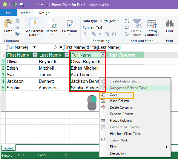
Click on the formula bar of the new column you just created and enter the following formula:
=[First Name]&" "&[Last Name]Hit Enter and Power Pivot will merge the data in the First Name and Last Name column to the Full Name column.

Right-click on the Full Name column and choose Copy from the context menu.

Go to your original worksheet and paste the content by pressing the hotkey Ctrl + Shift + V. This ensures you get clean text data instead of an Excel table.
Use Excel VBA
If you don’t wish to manually combine two columns in Excel, you must use Excel VBA. Here, you can use a simple script to automate the process.

Feel free to use this script for personal or professional purposes:
Sub CombineColumnsWithSpace()

Dim col1 As String, col2 As String, outputCol As String

' Get column 1 from user input
col1 = InputBox("Enter the cell reference for the first column (e.g., A:A)")

' Check if input is valid
If col1 = "" Then
    MsgBox "Please enter a valid cell reference.", vbExclamation
    Exit Sub
End If

' Get column 2 from user input
col2 = InputBox("Enter the cell reference for the second column (e.g., B:B)")

' Check if input is valid
If col2 = "" Then
    MsgBox "Please enter a valid cell reference.", vbExclamation
    Exit Sub
End If

' Get output column from user input
outputCol = InputBox("Enter the cell reference for the combined column (e.g., C:C)")

' Check if input is valid
If outputCol = "" Then
    MsgBox "Please enter a valid cell reference.", vbExclamation
    Exit Sub
End If

' Loop through each row and combine columns with space
Dim i As Long
For i = 1 To Cells(Rows.Count, col1).End(xlUp).Row

    Cells(i, outputCol).Value = Cells(i, col1).Value & " " & Cells(i, col2).Value

Next i

' Message box confirmation
MsgBox "Columns successfully combined in " & outputCol & ".", vbInformation

End Sub
The above script will help you create a VBA macro that asks for the following inputs:
- Sheet name
- First column, like
A:A - Second column, like
B:B - Destination column, like
C:C
So, you don’t need to modify any part of the above script.
Read How To Use The VBA Code You Find Online to learn how to create a VBA macro using the above script.
Use Office Scripts
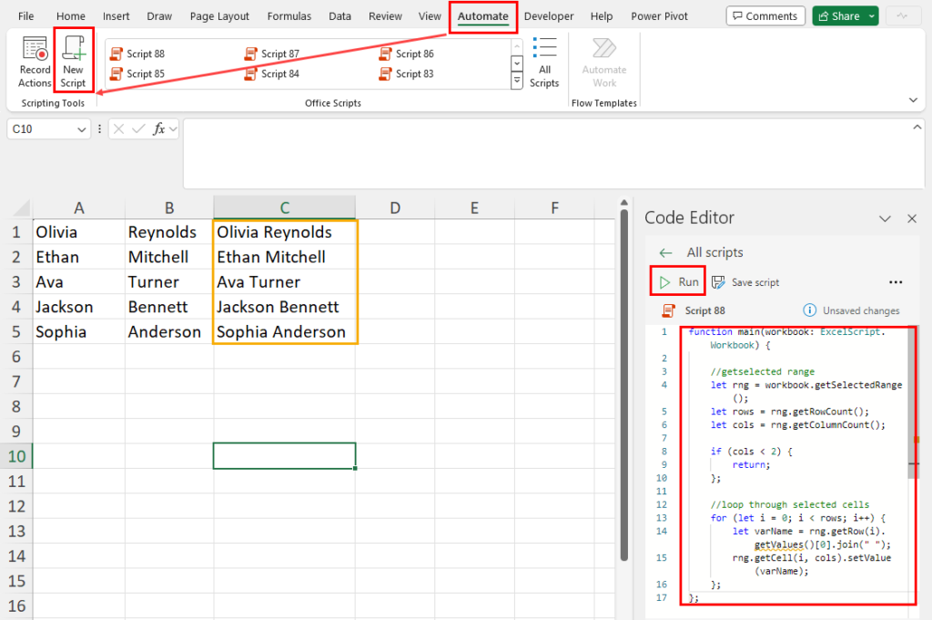
With Microsoft 365 Business Standard or a better subscription, you get Office Scripts for advanced automation in Excel. It’s specifically handy when you need to use Power Automate.

Here’s a script that you can use to automate the column-combining process in Excel:
function main(workbook: ExcelScript.Workbook) {

    //getselected range
    let rng = workbook.getSelectedRange();
    let rows = rng.getRowCount();
    let cols = rng.getColumnCount();

    if (cols < 2) {
        return;
    };

    //loop through selected cells
    for (let i = 0; i < rows; i++) {
      let varName = rng.getRow(i).getValues()[0].join(" ");
      rng.getCell(i, cols).setValue(varName);
    };
};
New to Office Scripts? No worries! Read this excellent article to learn how to create a shareable script using the above code:
Conclusions
So far, you’ve learned various methods to combine two columns in Excel.
Flash Fill and Notepad should be your first choice if you’re a new user of Excel spreadsheet software.
If you’re up to the challenge and looking to enhance your level to an intermediate Excel user, practice the functions-based methods like Equals and Ampersand, CONCAT, and TEXTJOIN.
Finally, if you consider yourself an Excel pro, you should use automatic and scaled-up methods like Power Query, Power Pivot, Office Scripts, and Excel VBA.
Don’t forget to comment below to share your feedback or tips.
 👉 Find out more about our Advanced Formulas course!


0 Comments