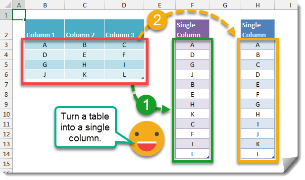
This post will explore how you can transform a table of values into a single column using the INDEX function.
Get your copy of the example workbook with the above link.
There are many ways you could transform a table into a single column but this post will explore the two ways that make the most sense.
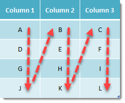
- Going down the rows first then across the columns in your table.
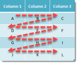
- Going across the columns first then down the rows in your table.

Here you have a table with 3 columns and 4 rows.
If you wanted to transform this into a single column of data you could start in row 1 column 1 and move down the rows until you reach the last row then move onto row 1 column 2 and start the pattern again until you cover the whole table like in the picture above.
=INDEX($B$3:$D$6,MOD(ROW()-ROW($F$2)-1,ROWS($B$3:$D$6))+1,INT((ROW()-ROW($F$2)-1)/ROWS($B$3:$D$6))+1)The above formula will produce a single column based on the top to bottom then right pattern.

Another approach could be to start in row 1 column 1 and move across the columns until you reach the last column then move down to row 2 column 1 and start the pattern again until you cover the whole table like in the picture above.
=INDEX($B$3:$D$6,INT((ROW()-ROW($H$2)-1)/COLUMNS($B$3:$D$6))+1,MOD(ROW()-ROW($H$2)-1,COLUMNS($B$3:$D$6))+1)The above formula will produce a single column based on the left to right then down pattern.
 👉 Find out more about our Advanced Formulas course!


0 Comments