Microsoft Excel is a Powerful Tool, Period.

And once you are loaded with all the basics of Microsoft Excel, it’s important for you to master the functions.

You must have heard a number of times that the power of Excel lies in its inbuilt functions and flexibility to create formulas as per your need and requirement.

One thing which I love the most about Microsoft TEAM that they keep on introducing new functions from time to time.

For Example: In the latest version of Excel i.e 2019/Office 365, they have introduced 6 New functions which can change the way you deal with the data.

Today in this post, I’d love to share those “6 New Excel Functions Introduced in Excel 2019/365“.

So let’s explore them one by one.

Video Tutorial

CONCAT Function

This function is an improvement over CONCATENATE.

How do you deal with the data when you have to combine a long list of cells to another list?

Let’s say you need to combine A1:A50 to B1:B50.

If you have been doing this using CONCATENATE in each and every cell, you need to stop and learn more about CONCAT.

This function allows you to combine text, strings or range into one string saving time and energy.

You can combine a string by just specifying the range and your work is done. There is no need to select each and every cell you want to join.

Syntax

CONCAT(text1,[text2],…)

• text1 can be a range, string or a reference cell to combine.
• text2 may or may not be required depending upon the nature of text 1.

Note: If text 1 is a range then text 2 is not mandatory.

Example

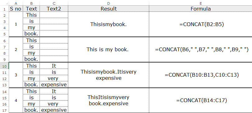
You can use CONCAT in several ways.

This function does not provide the delimiter argument so you need to define the spacing in the formula.

In the above examples, we have used CONCAT in different ways to combine values from a range.

TEXTJOIN Function

This function is similar to CONCAT but more powerful.

It joins multiple cells or ranges to one string with a specified delimiter. Yes, you can specify the delimiter or a separator in the function.

Remember if the delimiter is a number, it will be treated as a text.

Syntax

TEXTJOIN(delimiter, ignore_empty, text1, [text2], ...)

• The delimiter is actually the separator in your text. It should be defined in double quotes “”. It can be empty as well “”.
• ignore_empty can be TRUE or FALSE; if TRUE the function will ignore empty cells in your given ranges/text and vice versa.
• text1, text2, …textn are the text or ranges you wish to combine. Here n cannot exceed 252.

Example

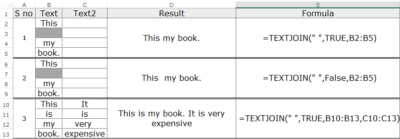
In the above examples, we have defined a delimiter as space ” ” which means all the text are separated by a space.

In the first example, we have specified TRUE to ignore empty values, therefore, the joined text returned by the function doesn’t have spaces.

But in the second example, it’s vice-versa.

And in the third example, we have combined two different ranges separated by the space and ignored empty cells.

Our result is different based on the ignore_empty command in all the above examples.

Don’t forget to check out some of the amazing tips on the concatenation:

• How to Conditionally Concatenate a Range
• 5 Ways to Concatenate Data with a Line Break in Excel
• How to Concatenate a Range with a Delimiter
• Summarizing Text Data with Pivot Tables

MINIFS and MAXIFS Function

MAXIFS and MINIFS return the maximum and minimum values respectively based on given conditions.

As the name describes, MAXIFS identifies the maximum value based on multiple conditions given in the formula and MINIFS returns the MIN value based on multiple conditions.

Both the functions support logical operators and criteria based on numeric, text or dates.

Syntax

MAXIFS(max_range, criteria_range1, criteria1, [criteria_range2, criteria2], ...)
MINIFS(min_range, criteria_range1, criteria1, [criteria_range2, criteria2], ...)

• max_range and min_range are the actual ranges in which the maximum or minimum value is determined. In other words, the range in which your answer lies is max_range or min_range.
• criteria_range1 is the set of the range which needs to be evaluated for condition 1 i.e criteria1.
• criteria1 is the actual condition to evaluate the maximum number. You can enter up to 126 conditions.

Note: The max_range/min_range and the criteria_range1 should be of same size else you will get an #VALUE error.

Example

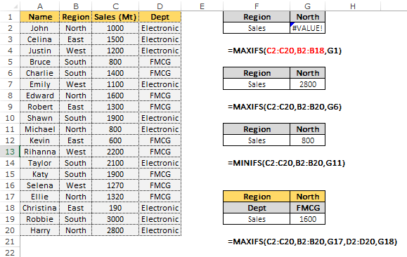
You can see in the above example, we are getting an error #VALUE! as the size of the criteria_range1 is different from Max_range.

The G2 column gives an error as the size of the ranges is different.

Also, refer the cell G19 where we have given 2 conditions Dept and Region.

Here, our maximum value lies in the range C2:C20 and our conditions are cells G17 and G18 which needs to be evaluated from ranges B2:B20 and D2:D20 respectively.

IFS Function

You might have been in a habit of typing long nested IF formulas if you are not aware of INDEX MATCH.

IFS is the solution to that.

This function checks the multiple conditions and returns the corresponding value.

Syntax

IFS(logical_test1,value_if_true1,[logical_test2, value_if_true2], ...)

Note: You can only include 127 combinations of logic and conditions.

• logical_test1 is the condition which needs to be evaluated.
• value_if_true1 is the result we need if logical_test1 is TRUE.
• logical test2 is the second condition and so on.

Note: IFS function does not have the ELSE condition like normal IF but you can create it by adding TRUE to the last logical test as mentioned in the example below.

Example

In the above example, we want the result to be “Excellent” if B2 >=90, “Good” if B2> =70, “Needs Improvement” if B2> =60, else we need the result to be “OTHER”.

Here we have created else statement by adding TRUE to the last logic.

And in the cell D9, we have used IFS without specifying ELSE argument.

SWITCH Function

This function helps you to evaluate your expression against the given set of values as IF function does.

It returns the value based on the first exact match.

Syntax

SWITCH (expression, value1, result1, [value2, result2], ..., [default])

• The expression is the argument or value to be compared against value1….value 126.
• value1 to value126 are the values which will be compared to our expression.
• default is the value returned when there is no match. You can change the default to text, sign, as per your choice.

SWITCH returns an error (#N/A) in case there is no match or there is no default value defined.

Remember, SWITCH function does not work with logical operators like, <, >, etc. It only evaluates character or an integer.

Example

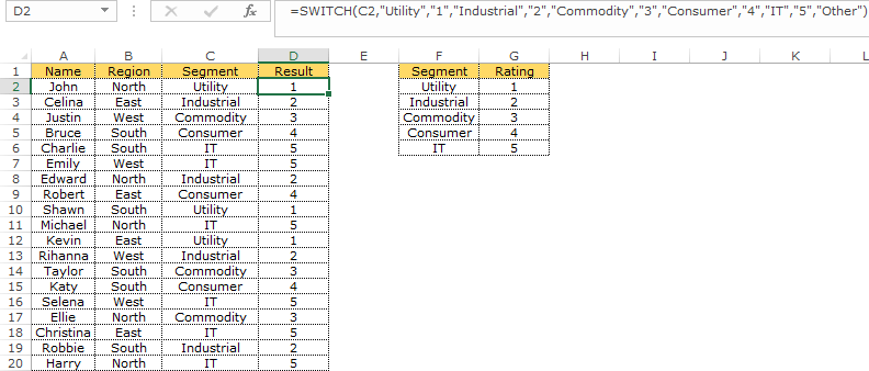
In the above example, C2 is the expression to be compared against our 5 segments to get the result i.e ratings.

=SWITCH(C2,"Utility","1","Industrial","2","Commodity","3","Consumer","4","IT","5","Other")

“Other” is the default value which will be returned in case no match found.

Sometimes you will feel SWITCH is just like a simple VLOOKUP.

In the End

Apart from these, there are more than 450 functions in Excel which you can use. But if you ask me you won’t need to learn all the functions.

You just need to master functions which are common in use + relevant to your work.

In his book “51 Excel Functions You Need To Know“, John has listed the top 51 Excel functions which every aspiring Excel user must learn.

Do you have any favorite Excel function which you use in your work?

Share with me in the comment section, I’d love to hear from you and please share this blog post with your friends.

About the Author

Aprajita Sharma

Aprajita is the Co-Founder of ExcelChamps. She has an MBA in Sales & Marketing and has been using Excel for the last 8 years. Her journey started from learning a basic pivot table from Google which made her fall in love with Excel. She is a lifeguard to people around the world who fight with data on a day to day basis.