Are the formulas on your Excel worksheet not calculating, updating, or working as intended? Keep reading to explore the sure-shot troubleshooting ideas to fix the Excel can’t calculate a formula error in no time!

Microsoft Excel is a powerful tool that has revolutionized the way you analyze and visualize data. Its one of powerful features is the ability to accept real-world formulas for mathematics, economics, statistics, and so on.

The formula feature is also the source of all sorts of errors in Excel. If you don’t use the syntax or arguments of a function the right way, it’ll surely generate an error message.

Such errors in Excel can annoy you when you need it the most. Fear not as you’ve landed on the right Excel tutorial to fix all sorts of formula calculation errors. Let’s get started!

What Is the Microsoft Excel Cannot Calculate a Formula Error?

This isn’t any single error but a collection of different errors. The most popular error when calculating a formula in Excel is the circular reference error. You’ll see the following message when there’s one:

Another error when creating an Excel formula you can face is Excel warning you about a potential problem with a function you just entered. In this situation, you get the following warning message:

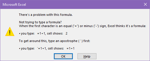
Find below other errors that might show up when you’re using various formulas in Excel and their definitions:

#DIV/0!

This error occurs when you attempt to divide a number by zero in your formula. Excel can’t perform division by zero. Hence, this action results in the “#DIV/0!” error. So, resolve such formula instances to fix this issue on one or many cells.

#VALUE!

The #VALUE! error indicates that you’re using the wrong data type within a formula. It can also occur when you’re trying to perform calculations with incompatible data types, such as adding text to a number.

#REF!

This error tells you that there’s an invalid cell reference within your formula. It usually occurs when you delete a referenced cell or range. Restore the referred cell address or range to fix the error.

#NAME

The #NAME? error occurs when Excel can’t recognize a function, formula, or named range referenced within a cell. It may be due to a misspelled function name or the absence of a necessary add-in.

So, double-check the function you used in your formula before pressing the Enter key. It’s better if you select the auto-suggested formula in Excel without typing it manually.

#N/A

The #N/A error stands for “Not Available.” It indicates that a value you’re looking for isn’t available within a lookup formula or a function that searches for specific data.

#NUM!

This error occurs when a formula produces a result that isn’t a valid number. It can happen with mathematical operations that yield extremely large or small numbers that exceed Excel’s capabilities.

#NULL!

This error arises when there’s an incorrect intersection of two ranges within a formula. It typically occurs when a space or comma is missing between range references.

Now that you know the various reasons why Microsoft Excel can’t calculate a formula, explore some common ways to fix this below:

Numbers Shouldn’t Be A Text String

Excel functions can’t include numbers during calculations if you format the numbers as text. Numbers formatted as texts might seem simple numbers to you but Microsoft Excel is unable to perceive those as numerical figures. Instead, it considers these as texts.

Here’s how you can know if numerical figures are in the text format or not:

• Excel will align normal numbers to the right side and numbers as text to the left side.
• You’ll see the Text option in the Number drop-down list on the Home tab for the selected number or cell.
• If there’s an accent symbol before a number in a cell, Excel will treat the value as text.
• If you see a green triangle in the top-left corner of a cell containing a numerical value, it’s in the Text format.

Find below an example of an Excel calculation error due to text formatting of numbers:

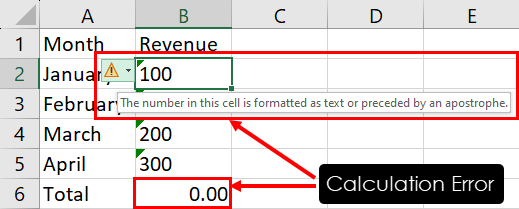
To fix the above issue, highlight all the cells within the column and click the error warning. On the context menu that opens, click Convert to Number. The SUM formula to the right of the Total cell will automatically show the sum of referenced cells.

Disable the Show Formulas Button

The Show Formulas button reveals the actual formula in each calculated cell instead of the resulting values. So, if you accidentally activate the Show Formulas button, you won’t see any values in any of the formula cells on your Excel worksheet.

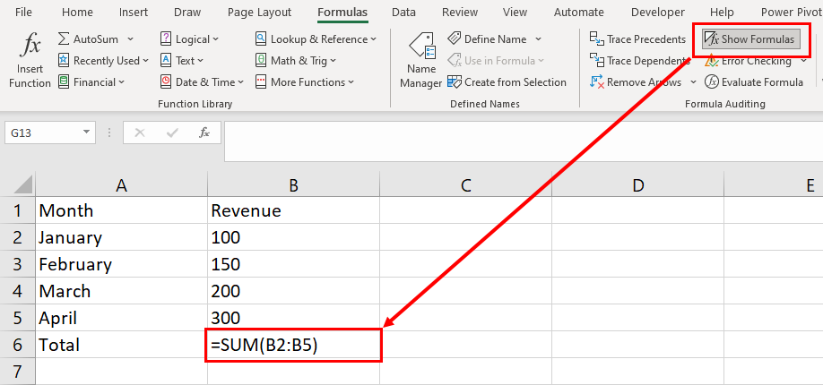
You’ll just see the raw formula. Seeing this you might think Microsoft Excel can’t calculate a formula. However, this is just a temporary setting of Excel and you can quickly fix this by following these steps:

1. Click the Formulas tab on the Excel ribbon menu.
2. Go to the Formula Auditing commands block.
3. Click the active (grey shade) Show Formulas button to deactivate it.

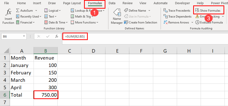
All the formulas in your worksheet will automatically calculate the formulas and show the resulting values.

Resolve Circular Reference Issues

The circular reference error pops up when you create an Excel formula that includes the cell reference of the formula itself. Here, you’re asking Excel to use the formula to calculate itself. Find below an example of a circular reference in Excel:

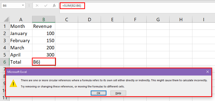
In the above scenario, the formula =SUM(B2:B6) is in the cell address B6. So, instead of getting a summation of the cell range B2:B5, the formula is trying to calculate itself.

It often happens when you use the keyboard to type the SUM references instead of manually selecting them using the mouse.

To resolve the above issue, click OK on the warning message. Then, closely inspect the formula to fix the cell references for the SUM function.

Now, your Excel worksheet may contain hundreds of such formulas. If any of these have a circular reference error, it’s truly challenging to manually check all the formulas. Instead, follow these steps to uncover circular references in Excel:

1. Click OK to close the warning.
2. Select the Formulas tab on the Excel ribbon menu.
3. Click the Error Checking drop-down menu inside the Formula Auditing section.
4. On the context menu that pops up, hover the mouse cursor over the Circular References option.
5. An overflow menu will show all the cell references where you should find the circular references.
6. Visit those highlighted cells and remove the reference to the formula cell to get rid of a circular reference error.

If you wish to automate the process of finding circular references in Excel, you can use this VBA script:

Sub FindCircularReference()
    Dim rngFormula As Range
    Dim cell As Range
    
    On Error Resume Next
    Set rngFormula = ActiveSheet.UsedRange.SpecialCells(xlCellTypeFormulas)
    
    For Each cell In rngFormula
        If cell.CircularReference Then
            MsgBox "Circular reference found at cell " & cell.Address
        End If
    Next cell
    
    On Error GoTo 0
End Sub

Here are the steps to use the above Excel VBA code:

1. Hit Alt + F11 to call the VBA Editor.
2. Click Insert and choose Module on the toolbar.
3. Copy and paste the above code.
4. Click Save and close the VBA Editor.

5. Press Alt + F8 to call the Macro dialog box.
6. Select the FindCircularReference macro and hit Run.

7. Excel will show a message box with all the circular reference cell addresses.

Use Allowed Characters and Symbols Only

In Excel, you must enclose functions within parentheses to define the arguments. In complex formulas, it’s common to use nested parentheses to specify the desired calculation order. However, it’s crucial to ensure the proper pairing of parentheses in your formula.

Excel assists in maintaining correct parenthesis pairs by displaying them in different colors as you enter them. If your formula is missing one or more closing parentheses, Excel will generate an error message and offer a suggestion to balance the pairs.

The following Excel function doesn’t have all the parentheses required to complete it:

=IF(A1>10,"Best",IF(A1>5,"Good",IF(A1>0,"Not Good","Fail"))

When executing this formula, you’ll get the following error:

Thankfully, the Excel program is intelligent enough to suggest you a fix. The correct formula is as mentioned below:

=IF(A1>10,"Best",IF(A1>5,"Good",IF(A1>0,"Not Good","Fail")))

Just like the parenthesis, you must also follow the following rules when constructing an Excel formula:

• Separate all the arguments of the functions with a comma (,).
• If you’re using the Excel app in the EU, you can use semicolons (;) to separate the arguments.
• If you’re referring to any workbook or worksheet in your formula containing non-alphabetical characters or spaces in their names, put them within single quotation marks, like =SUM('Sheet 1'!C2:C4).
• If using a number in a formula to represent a monetary value, don’t use a currency symbol like $. You can reformat the calculated cell with the Currency format later after the calculation is done. You can get this in Home > Number > General drop-down > Currency.

All the Required Arguments Must Be Present

When using an Excel function, you must enter values or reference cells for all the mandatory arguments. For example, for the following formula, [range_lookup] argument is optional but the rest are mandatory:

VLOOKUP(lookup_value, table_array, col_index_num, [range_lookup])

If you don’t enter the required values for any of the mandatory arguments, you get the following error message:

To avoid this issue, here’s how you should create a formula in Excel:

1. Double-click the target cell and type a few initial characters of the function you want.
2. When Excel suggests a list of functions in the context menu, double-click on the right one.

3. Once you select the function, Excel shows the full syntax of the function.
4. Read each argument carefully and enter values, cell references, variables, etc., one by one.

Choose an Appropriate Calculation Option

This is the least expected issue that you can face when working with functions in Excel. By default, all Excel desktop and web apps come with the Automatic choice for Calculation Options.

When you change this setting to Manual or Automatic Except for Data Tables, you might face the Excel can’t calculate a formula error. When you see that your Excel worksheet doesn’t recalculate formula cells after adding new values to the referenced cells, follow these steps to fix the issue:

1. Click the Formulas tab and go to the Calculation commands block.
2. There, click the Calculation Options drop-down arrow.
3. Choose Automatic if it’s Manual.

If your worksheet was in the Manual calculation mode, click the Calculate Now button on Formulas > Calculation section to force a recalculation instantly.

Conclusions

Working on Excel is fun. It’s even more enjoyable when you can successfully create a formula on your own or by following a tutorial online. Formulas make your life easier by solving complex mathematical or statistical problems in seconds.

If you just started using formulas in Excel or do this occasionally, it’s okay if you see various forms of Excel can’t calculate a formula error. Use the appropriate troubleshooting methods as explained above and fix all sorts of formula issues in a flash!