Do you need to combine both first and last names in Excel?

Adding a new column based on the joining of two columns is a basic task in data analysis. In data entry forms, most of the time the developer will keep two fields for first and last name instead of the full name.

It helps to avoid confusion, is easier to find, and will be very useful for further data analysis.

Suppose you are creating a report where you need to display a customer’s name. You will have to combine both names and display them as full names instead of keeping them separate.

There are a few different ways to combine data from two different cells into one cell. In this post, you will learn all the different methods to join names from two or more cells in Excel.

You can use the Ampersand operator, and in-built functions CONCATENATE, CONCAT, TEXTJOIN, and FLASH FILL to combine names.  Also, Power Query or Power Pivot can merge your names. If you want to combine names in your automation you can use either VBA or Office Scripts.

Get your copy of the example workbook used in this post to follow along!

Combine Names with an Ampersand Operator

The ampersand operator & can be used in Excel to combine two or more strings of text together. So you can use this to join your first and last names.

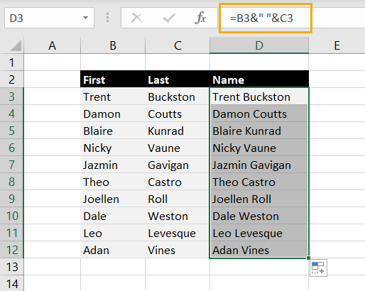
Suppose you have First Names and Last Names in the range B3:B12 and C3:C12 respectively.

= B3 & " " & C3

You can use the above formula to concatenate them in cell D3 and drag the fill handle to apply the formula to the range of cells D3:D12.

This adds a space between first and last names in the above example. If you want you could add any other character or delimiter such as a comma.

Combine Names with the CONCATENATE Function

You can use a simple CONCATENATE formula to combine data from two or more cells into one cell. This is useful if you need to create full names.

CONCATENATE ( text1, [text2], ... )

The CONCATENATE function takes one or more text values and combines them within one value.

📝 Note: The CONCATENATE function can only take a cell reference as an argument and will not combine all the text in a range reference. This means you have to reference each cell individually.

= CONCATENATE ( B3, " ", C3 )

The above formula will combine the data from cells B3 and C3 along with a space character between them.

📝 Note: You need to specify the space character in between the names as the CONCATENATE function will combine the arguments in the order they appear.

Combine Names with the CONCAT Function

The CONCAT function allows you to combine the text from multiple ranges into one cell.

This is a useful function when you have data in multiple adjoining cells and you want to combine them into one cell for use in a formula or for display purposes.

CONCAT ( text1, [text2], … )

The CONCAT function accepts multiple ranges of text cells instead of needing to select each cell individually.

The following example shows how to use the CONCAT function to combine first and last names.

= CONCAT ( B3:D3 )

The CONCAT function will combine the data from the range of cells you specified and display the combined data in the cell you selected.

Please note that you have added a single space in Column C in the above example. Otherwise, Excel will join the names into a single name.

📝 Note: You have to add a single space in a column between your first and last name columns. Otherwise, Excel will join the names into a single text without a space to separate them.

Combine Names with the TEXTJOIN Function

The TEXTJOIN function allows you to combine text from multiple cells into a single cell with a delimiter between the text.

This will allow you to join the names with a space without the need to add an extra column containing a space character.

You also have the option to ignore empty cells. This way, any data with the first or last name missing won’t create a name with a trailing or leading space.

TEXTJOIN ( delimiter, ignore_empty, text1, [text2], … )

• delimiter is the character or set of characters you want to separate each joined text value.
• ignore_empty allows you to ignore any empty cells when joining text.
• text is the range of cells you want to join together.

= TEXTJOIN ( " ", TRUE, B3:C3 )

The above formula will join the names in the range B3:C3 and place a space character between them.

The first argument in this function is the delimiter. This is what will separate the text in each cell, so a single space character is used here.

The TRUE value is used to ignore any potential empty cells. In this case, there are no empty cells in the name data, so this argument will have no effect.

Combine Names with the Flash Fill Function

Excel Flash Fill is a feature that allows you to quickly fill in data based on examples that you enter.

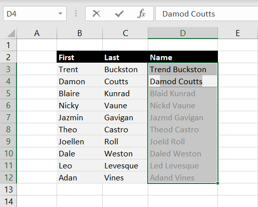
You provide a few examples of the results you want in the adjacent rows and Flash Fill will determine the pattern and fill in the rest.

Suppose you have a list of first and last names, you can use Flash Fill to quickly generate a list of full names.

Type the example full name into the cells to the right of the corresponding first and last name.

This should trigger Flash Fill and you will see the suggested results in light gray. Press Enter to accept these results and place them into the cells.

If Flash Fill does not trigger automatically after the first couple of entries, then you might need to manually trigger it.

Follow the below steps to manually trigger the Flash Fill

1. Select the first empty cell below your example Full Name.
2. Go to the Data tab.
3. Click on the Flash Fill command icon found in the Data Tools section.

💡 Tip: You can also use the Ctrl + E keyboard shortcut to trigger flash fill.

Combine Names with Power Query

Excel Power Query is a tool that allows users to easily extract and transform data from various sources such as databases, web pages, and text files.

It can also be used to transform and clean data before it is loaded into Excel.

This can be used to combine names in excel.

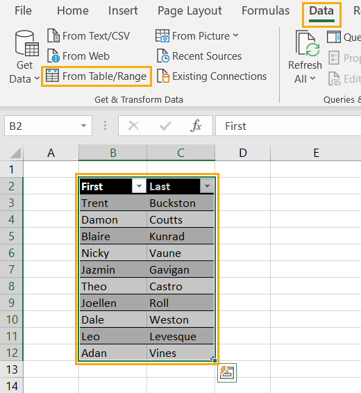
You will first need to add your name data into an Excel table.

Suppose you have data of first and last names in an excel table, then you can follow these steps to combine the names into a single column using Power Query.

1. Select your Excel table.
2. Go to the Data tab.
3. Choose the From Table/Range option.

This will open the Power Query editor window.

Now you can see your excel data table in the Power Query editor

4. Select both columns.
5. Right-click on the column headings.
6. Select Merge columns from the menu.

This will open the Merge Columns dialog box.   

6. Choose the Space option in the Separator dropdown menu. You can select from other options in the drop-down, or you can add your own custom delimiter.
7. Give your new column name in the New column name (optional) input box. For example, FullName.
8. Press the OK button.

You can see the first and last names are combined with a space between them in a new column named FullName.

9. Press Close and Load to in the Home tab.

Excel will close the Power Query Editor and the Import Data dialog box will open.

10. Choose the Existing worksheet, If you need to import data in a new worksheet you can select the New Worksheet option instead.
11. Select any cell such as E2.
12. Press the OK button.

The combined names will now appear in the output column in your excel.

Combine Names with Power Pivot

Excel Power Pivot is a data analysis tool that allows users to manipulate large data sets in Excel.

Power Pivot allows users to create pivot tables and charts from data that is stored in multiple tables.

After you load your dataset to the Power Pivot data model, you can add more columns with calculations using the DAX formula language.

The DAX formula language has a lot of common functions with Excel and in this case, you can use a simple ampersand & operator to combine names.

Suppose you have data in an excel table B2:C12 and need to add the data to the data model.

Select a cell inside the table that contains your First and Last names and go to the Power Pivot tab then click on the Add to Data Model option.

📝 Note: If you don’t see the Power Pivot tab in your Excel, you might need to enable the Power Pivot add-in first.

This will open the Power Pivot editor with the table loaded to the model.

You will be able to add new columns by clicking on the Add Column heading to the right of your data.

= [First] & "  " & [Last]

The above formula will give the combined names for the entire column.

Now you will be able to use these calculated columns in a Pivot Table.

Go to the Home tab of the Power Pivot Add-In and click on the PivotTable command and choose the PivotTable option from the menu.

This opens Create PivotTable dialog box. Choose either New Worksheet or Exiting Worksheet. Give the cell location where you need to add the pivot table and press the OK button.

You can see the empty pivot is added in your excel and the calculated column FullName is available in your PivotTable Fields list. When you add this to your pivot table Rows area, you’ll see a list of full names combined in one column.

Combine Names with VBA

Excel VBA is a programming language that enables you to control Excel using code.

You can use VBA to write macros, create user forms and controls, and automate most processes. VBA is built into Excel, and you can access it using the Visual Basic Editor.

You can add a macro to your workbook that will combine the names into adjacent columns.

This can be run by adding the macro to the Quick Access Toolbar so it’s always available to use in one click.

Access the VBA editor and add the code

Go to the Developer tab and click on the Visual Basic command.

You can check out this post for details on enabling the Developer tab in the ribbon. Alternatively, you can press Alt + F11 to open the visual basic editor without the Developer tab.

This will open the visual basic editor. Now you can create a new module in the editor to add your code into.

Go to the Insert menu of the visual basic editor and select the Module option. It will add a new Module to your Modules folder

Sub CombineNames()
Dim rng As Range
Dim arrNames() As Variant
Dim colCount As Long
Dim rowCount As Long

Set rng = Selection
rowCount = rng.Rows.Count
colCount = rng.Columns.Count
ReDim arrNames(colCount)

If colCount < 2 Then
    MsgBox ("Select at least two columns!")
    End
End If

For i = 1 To rowCount
    For j = 1 To colCount
        arrNames(j) = rng.Cells(i, j).Value
    Next j
    rng.Cells(i, colCount).Offset(0, 1).Value = Trim(Join(arrNames, " "))
Next i
End Sub

Add the above code to your module in the visual basic editor.

This code first checks that you have selected a range with more than one column. If you have selected only one column it will warn you to select at least two columns and then stop execution.

When two or more columns are selected, the code will loop through the selected range and combine each cell with a space character.

It stores the First and Last names in an array object arrNames, Joins the array element with a space character and enters the data into the cells directly to the right of your original selection.

After you select your names and run the code, you will have the combined Full Name in Excel.

Combine Names with Office Scripts

Microsoft Excel Office Scripts allows users to record macros in Excel online and save them as Office Scripts. These scripts can be run in online excel to automate your tasks.

Go to the Automate tab and click on the New Script command to open the Code Editor for Office Scripts

function main(workbook: ExcelScript.Workbook) {

    //getselected range
    let rng = workbook.getSelectedRange();
    let rows = rng.getRowCount();
    let cols = rng.getColumnCount();

    if (cols < 2) {
        return;
    };

    //loop through selected cells
    for (let i = 0; i < rows; i++) {
      let varName = rng.getRow(i).getValues()[0].join(" ");
      rng.getCell(i, cols).setValue(varName);
    };
};

Add the above code to the Code Editor and press the Save button.

Now you can select at least two columns of names in your Excel sheet, Select your script combineNames from the Office Scripts drop-down items, and press the Run button found in the Code Editor.

The code will check your selection to ensure you have selected at least two columns. The code stops running otherwise. Otherwise, the code will continue and loop through your selected cells and combine the names in each row of your selection.

Conclusions

When you have two separate name fields for first and last names, you might need to join both names into one field with a space character between them. Thankfully, there are many ways to get this done.

A formula solution is the most dynamic and is better suited when names are added or updated to the original set of data.

Flash Fill will do the job in a few simple steps and is suitable for one-time operations.

The Power Query or Power Pivot approach is suitable for bigger datasets or external datasets.

You can use either VBA or Office Scripts method to combine names if you need to add this step to your automation.

Do you know any other method to combine names in Excel? Let me know in the comments section!