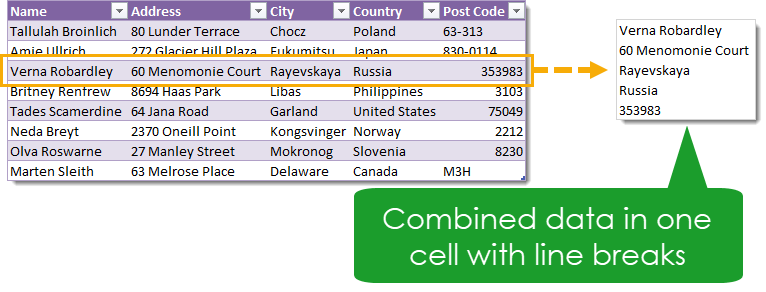
My girlfriend recently wanted to create printable address labels in Excel. She had a table of contact information including the name, street address, city, country and postal code for each person.

The problem was that she needed to display the name, street, city, country and post code each on a separate line within one cell.

In this post we’re going to take a look at five different ways we can concatenate the data and separate each item with line breaks. In other words, we will combine or join data from multiple cells into one cell and separate them with line breaks.

In all these methods, our data is contained in an Excel Table called Contacts.

Download the sample workbook to see all the solutions.

Concatenate with Line Breaks Using the Ampersand Operator

This is the most basic method, and if you have a small number of columns then it’s easy to set up.

The idea is we will use the ampersand operator & to join our data. This concatenates cells or text strings when used in a formula.

We will also need to use the CHAR function. This function converts an integer number from 1 to 255 into a unicode character. In fact, CHAR(10) will return the desired line break character. We will be using this in all of the formula methods in this post to create a line break character.

=A2&CHAR(10)&B2&CHAR(10)&C2&CHAR(10)&D2&CHAR(10)&E2

This formula is quite simple. It alternates between joining an item from the address to a line break character created from the CHAR function.

Concatenate with Line Breaks Using the CONCATENATE or CONCAT Function

This method is the essentially the same as the & method, but instead we can use either the CONCATENATE or CONCAT functions.

CONCATENATE and CONCAT functions do almost the exact same things, but CONCAT allows you to reference a range instead of individual cells like the CONCATENATE function. We can use either since our solution will only use single cell references.

=CONCATENATE(A2,CHAR(10),B2,CHAR(10),C2,CHAR(10),D2,CHAR(10),E2)

Again, the formula alternates between referencing the data and a line break character. It’s almost the exact same formula if you want to use the CONCAT function instead. Just replace CONCATENATE with CONCAT.

Concatenate with Line Breaks Using the TEXTJOIN Function

This is another formula method, but it’s the preferred way if you’re dealing with combining many columns into one cell. The previous methods become very tedious to write out the formula when we have more than a few columns.

The TEXTJOIN formula is perfect for joining data in a range and separating them with a delimiter character. In our case, we will use a line break character as the delimiting character.

=TEXTJOIN(CHAR(10),TRUE,A2:E2)

Now we can reference the data all in one range, instead of individual cells like the previous two formulas. We also only have to define the delimiter once in the formula.

Concatenate with Line Breaks Using a Power Query

Power Query is such an awesome data transformation tool. Nowadays, whenever I come across a problem, I always think about how I can solve it using power query.

Since this problem is a data transformation problem, power query can definitely do it.

Select the table of address data and go to the Data tab and choose the From Table/Range command.

We need to make sure all the fields are text type. We will later be concatenating them with a Text.Combine function and this will cause an error if any of the fields are not text type.

Notice that the postal code field contains both text and numbers, and has been given a generic data type as a result. Left click on the data type icon and select Text from the options to change this.

Now we are ready to add a new step to combine the data. Click on the fx icon next to the formula bar in the power query editor to add a new step. The new step will show the reference to the previous step (something like #"Changed Type"). We can remove this but take note as it will need to be used in the formula we input.

= Table.AddColumn(#"Changed Type", "Address Labels", each Text.Combine(Record.ToList(_),"#(lf)"))

Paste the above formula into the formula bar and press Enter to confirm the new step.

This formula will create a new column in the data where each row is the result of concatenating the data from the other columns with the power query line break character #(lf).

Now we can Close and Load the data from the Home tab.

Concatenate with Line Breaks Using DAX and Power Pivot

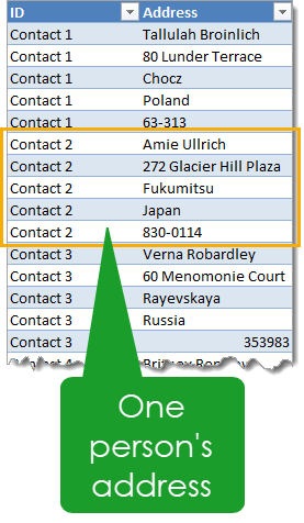
In order to use a pivot table to combine our data, we’ll need it in a slightly different format. We need to have all the address data in one column and another column which identifies the data as relating to each other.

With our data in this format, we can create a new pivot table. Select the data and go to the Insert tab and press the PivotTable command.

In the Create PivotTable dialog box, make sure to check the Add this data to the Data Model box. This will allow us to create measures using the DAX fomula language within out pivot tables.

In the PivotTable Fields window, right click on the table name and choose Add Measure.

=CONCATENATEX('ContactList','ContactList'[Address],"
")

Add a Measure Name like Label,then enter the above formula for the measure and press the OK button.

Notice that the line break character needed in the measure formula is actually a line break? You can create this in the formula editor by pressing Enter while inputting a formula.

We should now see a new field listed in the PivotTable Fields window. It will have a small fx icon next to it to indicate that it’s a measure.

We will now build our pivot table to display the address information in one cell per person. Drag the ID field into the Rows area and the Label field (measure) into the Values area.

Formatting the Results with Wrap Text

Ok, you may be thinking to yourself “I did all the steps, but I’m still not seeing the results. The data appears to be all on one line still!”.

Trust me, the line break characters are there. We need to format the cells to wrap text in order to see the results.

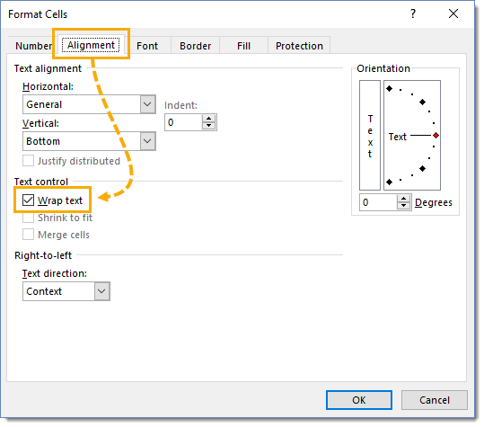
Select any cells you want to format and right click and choose Format Cells from the options. You can also press Ctrl + 1 on your keyboard to open the Format Cells dialog box.

Go to the Alignment tab and check the Wrap text box and press the OK button.

The cell will now display on multiple lines.

Conclusions

Excel has many options to combine data into a single cell with each item of data on its own line.

Most of the time using a formula based solution will be the quickest and easiest way.

We may find ourselves in need of an option which can’t easily be accidentally changed. Power query and power pivot is more suitable in this case.

Whatever the solution, it’s always good to know about all your options.