Excel Options

Excel has a lot of default options. You can find these all in the Excel Options menu.

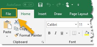
Go to the File tab.

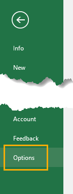
Select Options from the File menu.

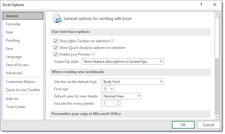
This will open up the Excel Options menu where you can find all of Excel’s many different settings options. The left hand side of the dialog box contains tabs to organize the various options into different categories and the right hand side is where you can adjust the settings.

This is a valuable tip in itself, but we will explore some of the more useful options later on.

Remove Gridlines from a Sheet

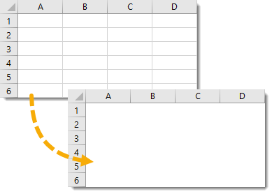
For a much cleaner and more modern look to your worksheets, remove the grid lines from any worksheet.

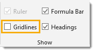
Go to the View tab in the ribbon then deselect the Gridlines options in the Show section of the ribbon.

Change the Gridline Colour for Any Sheet

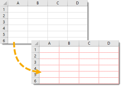
It’s possible to change the gridline colour from the default grey to a variety of other colours. This can be found in the Excel Options menu.

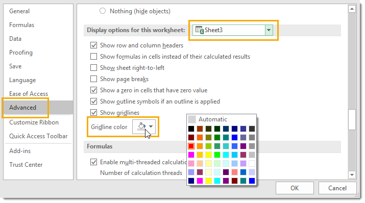
In the Excel Options menu go the the Advanced settings, then scroll down to the Display options for this worksheet.

Select the worksheet from the drop down menu for which you want to change the gridline colour. Now click on the Gridline color option and select a colour and press the Ok button.

Easily Rename a Worksheet

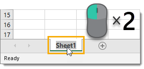
When you create a new sheet Excel will automatically give it a sequential name like Sheet1, Sheet2, Sheet3 etc. You can quickly rename any sheet with a double left click on the sheet’s tab in the lower left area of the workbook. Then you can type a new name and press Enter to complete it.

Insert a New Worksheet

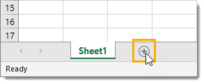
The quickest way to add a new sheet into a workbook is to left click on the small plus sign to the left of all the sheet tabs.

You can also insert a new sheet from the Home tab then Insert then Insert Sheet or by using the Shift + F11 keyboard shortcut.

Navigate Through Your Sheets

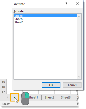
If you end up with a lot of sheets in your workbook, navigating through them can become difficult. There is an easy navigation method available.

Right click on either of the small arrows to the left of all the sheet tabs. This will open up the Activate, and you can select any of the worksheets listed then press the Ok button to go to that sheet.

Select the Entire Sheet

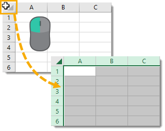
The intersection of the column and row headings is actually a button. You can select the entire worksheet by clicking on it.

Double Click to Autofit Column Width

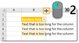
You can automatically adjust the column width to fit the data it contains. Hover your mouse cursor over the column border until it changes to a line with two arrows then double left click.

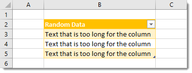
The column width will adjust so that all data in the column fits. This trick will also work for automatically adjusting row height.

Display Numbers in Thousands or Millions with a Custom Number Format

Display numbers as thousands using the custom format code 0.0, "k".

Display numbers as millions using the custom format code 0.0,, "M".

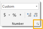
Highlight any cells you want to format then open the Format Cells dialog box by going to the Home tab and then clicking on the small icon in the lower right corner of the Number section. You can also use the Ctrl + 1 keyboard shortcut.

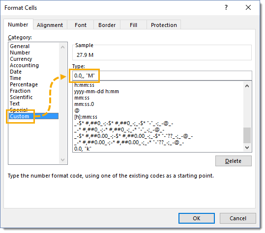
Go to the Number tab in the Format Cells dialog box and then select Custom under the category. Enter the custom format and press the OK button.

Invisible Data with a Custom Number Format

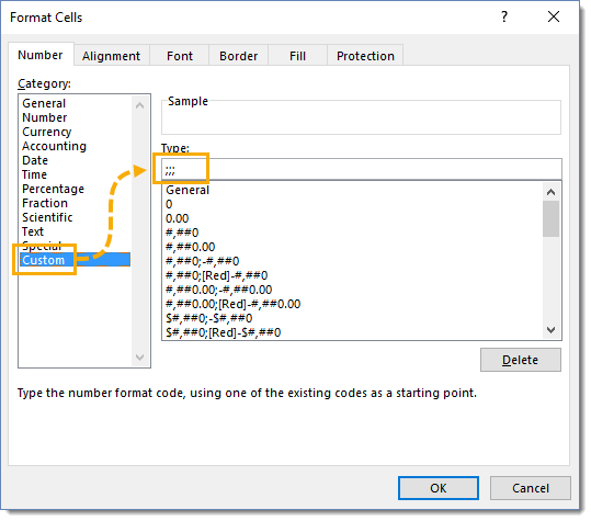
You can format data so that it is invisible on the worksheet. It will not be visible in the worksheet, but will be visible in the formula bar when the active cell cursor is on the cell.

Select any cells you want to hide and press Ctrl + 1 to open the Format Cells dialog box. Go to the Number tab and select Custom from the category. In the Type input put three semi-colons ;;; and press the OK button.

Now your data will not show on the sheet!

Remember though, the data is still there and can be seen when the active cell cursor is on that cell, don’t hide anything sensitive and think it will be safe.

Quickly Copy a Sheet with Ctrl and Drag

The regular method of making a copy of a sheet is slow.

You need to right click on the sheet you want to copy then select Move or Copy from the menu. This will open the Move or Copy dialog box. Then you will need to check Create a copy box and select where the new copy should appear.

There’s room for improvement.

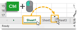
You can make a copy of any sheet easily by holding Ctrl and dragging the sheet. The arrow icon should show a small sheet with a plus sign. You can then release it to its new location to create the copy.

Insert Numbers as Text to Retain Leading Zeros

Have you ever tried to enter a serial number like 000135694 into Excel? The leading zero’s will disappear because Excel will automatically convert this to a number. It can be frustrating if you don’t know how to keep the zero’s.

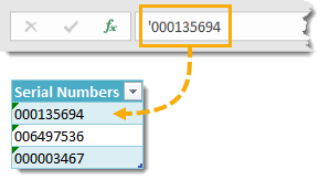
You can enter an apostrophe as the first character in the cell. This will tell Excel to treat the entry as text and the leading zero’s will be retained.

Automatically Open All Files in a Folder on Startup

Do you constantly use the same couple of files in Excel? Every time you start up Excel, you can have all these files automatically open for you!

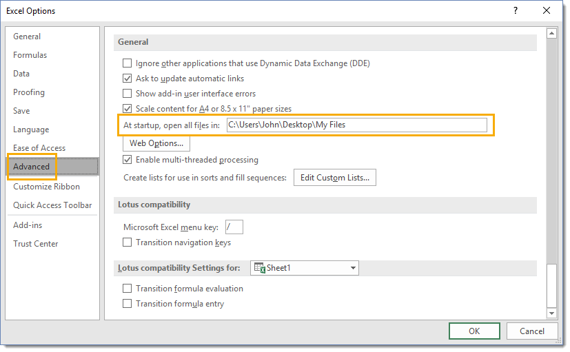
Open the Excel Options and go to the Advanced tab then scroll down to the General section. Set the path of the folder which you want to open files from in the At startup, open all files in input box.

If you want to keep the files saved elsewhere, you can simply add file shortcuts to this folder instead of storing the file there.

Now when you start Excel, all the files in this folder will automatically open.

Hide the Ribbon

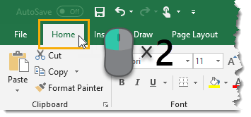
You can create a bit more worksheet real estate by hiding the ribbon commands. This can be quickly done with a double left click on any of the ribbon tabs. Double left click again to show the ribbon commands.

This can also be performed with a right click on any of the ribbon tabs and then selecting Collapse the Ribbon from the menu.

Enable the Hidden Developer Tab

There’s an extra tab in the command ribbon that’s disabled by default. It’s the Developer tab. If you want to start recording macros or writing VBA code to automate tasks, then it’s essential to enable it.

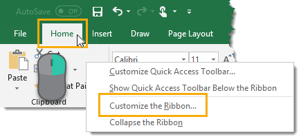
Right click anywhere in the ribbon and select Customize the Ribbon from the menu.

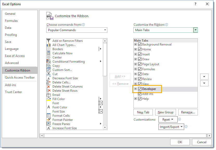
Check the box next to the Developer tab in the Main Tabs and then press the OK button. The new tab will now appear in your ribbon.

Very Hidden Sheets

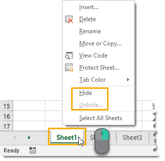
It’s possible to hide sheets by right clicking on the sheet tab and then selecting Hide from the menu.

But a user can easily unhide any hidden sheets also by right clicking on any sheet tab and then selecting Unhide. Then a list of all hidden sheet in the workbook are displayed for the user to select and unhide.

We can create Very Hidden sheets from within the Visual Basic Editor that users won’t be able to unhide.

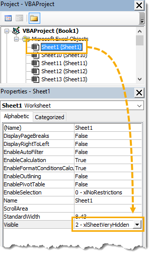
Open the Visual Basic Editor from the Developer tab or by using the Alt + F11 keyboard shortcut.

Find the sheet in the project explorer which you want to hide and select it. Then select xlSheetVeryHidden from the Properties window pane.

Resize Your Formula Bar

If the data or formulas in your spreadsheet start to get really long, then they might appear cut off in the formula bar.

You can resize the formula bar vertically or horizontally by clicking and dragging along the horizontal edge or between the name box and formula bar. When you hover the mouse over these areas the cursor will change to a two way arrow.

You can then use the quick collapse and expand toggle to quickly switch between the one line size and the expanded size. You can also use the Ctrl + Shift + U keyboard shortcut to toggle the formula bar size.

Using Union and Intersect Operators in Formula

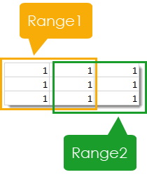
Using a comma between ranges in an array formula like SUM(Range1,Range2) will sum all the cells in all the ranges. This is like taking the union of all the ranges. In our example this would result in 12.

Using a space between ranges in an array formula like SUM(Range1 Range2) will sum only the common cells in all the ranges. This is like taking the intersection of all the ranges. In our example this would result in 3.

Create a Named Constant

With named ranges, you can name a cell and then store a constant value in that cell which will allow you to refer to a constant value in formulas throughout your spreadsheet.

You don’t actually need to store the value in a cell. You can create a named constant instead of using a named range.

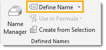
Go to the Formulas tab and use the Defined Name command found in the Defined Names section.

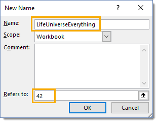
Now give your constant a Name and add your constant value in the Refers to section.

Now you’ll be able to use the constant in any formula and there is less chance the constant will be accidentally changed when using the spreadsheet.

Entering and Displaying Fractions

Did you know you can enter and display fractions in Excel? Yes, you can! Add a leading zero or integer followed by a space then the fraction part. The cell will display as a fraction but the value shown in the formula bar will be the equivalent decimal value.

• Enter 0 1/2 for the value 0.5
• Enter 2 3/4 for the value 2.75
• Enter 1 1/2 for the value 1.5

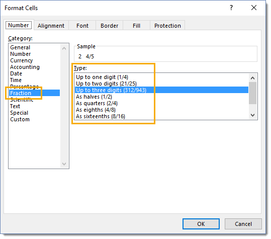
You can also format any decimal number you’ve entered as a fraction by going to the Format Cells dialog box (Ctrl + 1 is the keyboard shortcut) and selecting Fraction as the category.

Using Tilted Headings

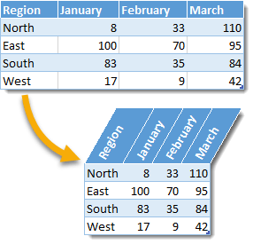
Make your reports look super cool and save valuable column width by using tilted headings

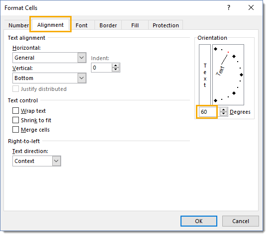
Select the cells you want to tilt then open up the Format Cells dialog box using the Ctrl + 1 keyboard shortcut. Go to the Alignment tab and change the Orientation to the desired angle.

Explore Get & Transform Data (Power Query)

Do you work with data from many different sources, or with poorly formatted data that you’re constantly needing the clean before using? Then you need to check out Power Query!

Power query is an ETL tool (Extract, Transform and Load) that’s built into Excel since 2016 and it’s extremely useful for getting your data into Excel in the format you need it in.

Check out my introduction to power query to learn more about this amazing tool.

Add Split Bars to a Worksheet

Have you ever wanted to view multiple locations in a sheet at the same time? Then you need to add split bars to your worksheet.

This will add a cross bar into your worksheet area that will allow you to independently scroll around the sheet in 4 different quadrants.

Go to the View tab and press the Split button.

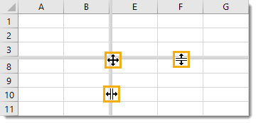
You can click and drag either of the split bars around as needed or click and drag the center to move them simultaneously.

Double left click any part of the bar to remove them from the sheet.

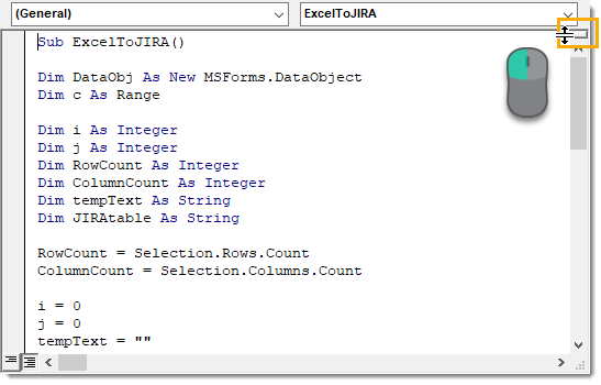
There’s even a split bar in the visual basic editor if you need to view two parts of your code at the same time. It’s located at the very top of the scroll bar. Drag it into place or double left click on it to insert it.

When you’re finished with it, drag it back to the top or double left click on the bar to remove it.

Select All Cells Containing a Specific Text String

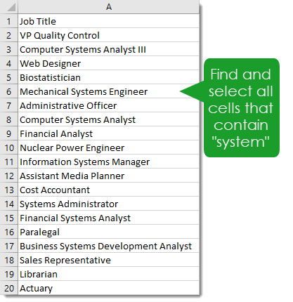
You can use Excel’s Find & Select to select all cells in a worksheet that contain a given keyword.

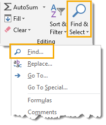
Open the Find and Replace dialog box by going to the Home tab and pressing the Find & Select button in the Editing section of the ribbon, then choose Find from the menu.

You can also open this using the Ctrl + F keyboard shortcut.

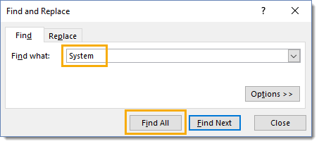
Now you can enter the string of text or numbers you want to find and press the Find All button.

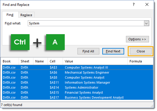
This will bring up a list of cells where the searched text string was found. Now if you can press Ctrl + A to select all the results. This will also select the cells in the workbook and when you press the Close button the cells in the workbook will remain selected.

Add a Line Break Inside a Cell

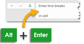
If you want to make text in a cell a bit more readable add in some white space by using Alt + Enter to add in line breaks within the cell. This will allow you to format text into a more readable paragraph structure that people are used to seeing.

You can also add line breaks in text created with formulas. Try this example ="First line"&CHAR(10)&"Second line".

Search for all Cells with a Line Break

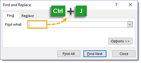
You can search for all line breaks in a sheet.

Open up the Find and Replace window either from Home > Find & Select > Find or using the Ctrl + F.

Place the cursor in the Find what field and press Ctrl + J. This will enter a line break character into the search criteria field. You won’t be able to see it, but it’s there. Now press either the Find All or Find Next button to search.

Close All Workbooks

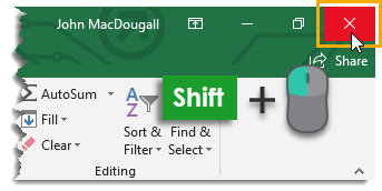
If you have a lot of workbooks open and you want to close them all at once, there’s a quick way to do it.

Hold Shift while clicking on the X in the top right of a workbook. This will save having to individually click on the X in each workbook!

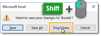
If some of the workbooks you’re closing have unsaved changes then you’ll get a pop up asking if you want to save changes for each of them. There’s no button for “Don’t Save All“. However, if you hold Shift and click on Don’t Save then you won’t be asked again for any of the other files.

Navigate Excel Using the Name Box

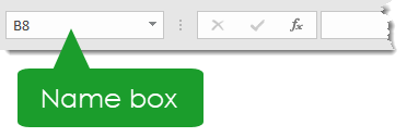
Use the Name Box to navigate around the active sheet. You can type any cell address like C420 into the name box and when you press Enter, you’ll be taken to that cell. This is great for moving to far away cells.

This isn’t as useful, but you can also navigate to other sheets. You need to type out the full cell address including the sheet name like 'Other Sheet'!D18.

It is also possible to navigate to any named range in the workbook with the name box. Click on the small arrow on the right side of the name box and select the named range from the drop down menu.

Using the Function Tooltip

When typing a function into a cell, Excel will display a function tooltip bar which shows the required and optional arguments for the function.

If the tooltip gets in the way, you can move it. Hover the cursor over the edge of the tooltip until the cursor changes to a four way arrow, then you can click and drag the tooltip to a new location out of the way.

If you click on the function name in the tooltip, it will open the functions help topic on Microsoft’s support website.

If you click on one of the function’s arguments in the tooltip, it will select that part of your function.

Turn Off the Function Tooltip

If you find the function autocomplete too annoying and you don’t want to see if ever then you can turn it off.

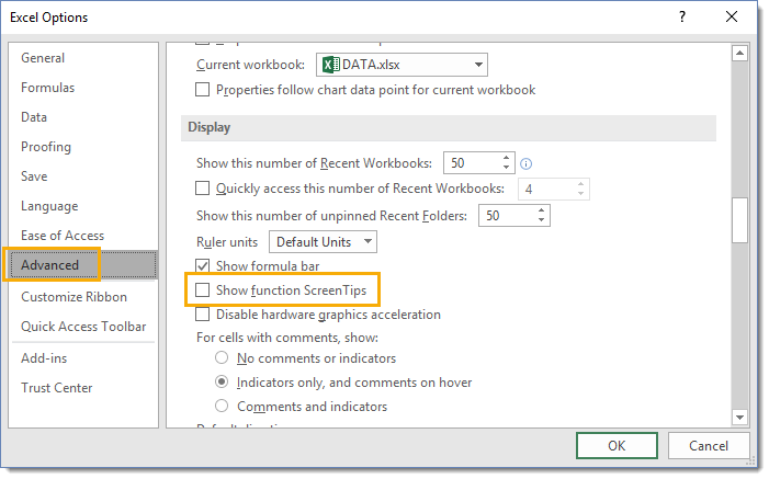
Open the Excel Options and go to the Advanced tab then scroll down to the Display section and uncheck the Show function ScreenTips box.

Set a Workbook to Always Open on a Specific Sheet

Excel will open a workbook to the sheet that was active when the workbook was last saved.

If you want to set up your workbook to always open on a specified sheet regardless of what sheet was active when it was saved, then add this bit of code into the workbook’s visual basic editor.

Sub Workbook_open()
    ActiveWorkbook.Sheets("My Start Sheet").Activate
End Sub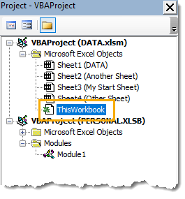

Press Alt + F11 to open the visual basic editor and copy the code into ThisWorkbook Excel Object. Change “My Start Sheet” to the name of the sheet in your workbook.

Add a Word to the Spell Check Dictionary

Maybe your company name isn’t a real word but it’s appears throughout your spreadsheets and you don’t want it to be flagged by Excel’s spell check every time. You can add it to the dictionary.

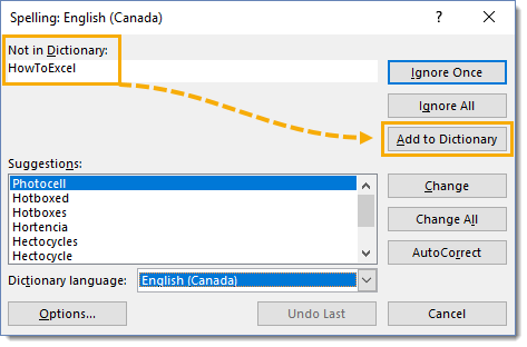
You can add words one by one as they get flagged by the spell check. Go to the Review tab and press the Spelling command to start the spell check. When a word is flagged by the spell check press the Add to Dictionary button and the spell check will ignore it going forward.

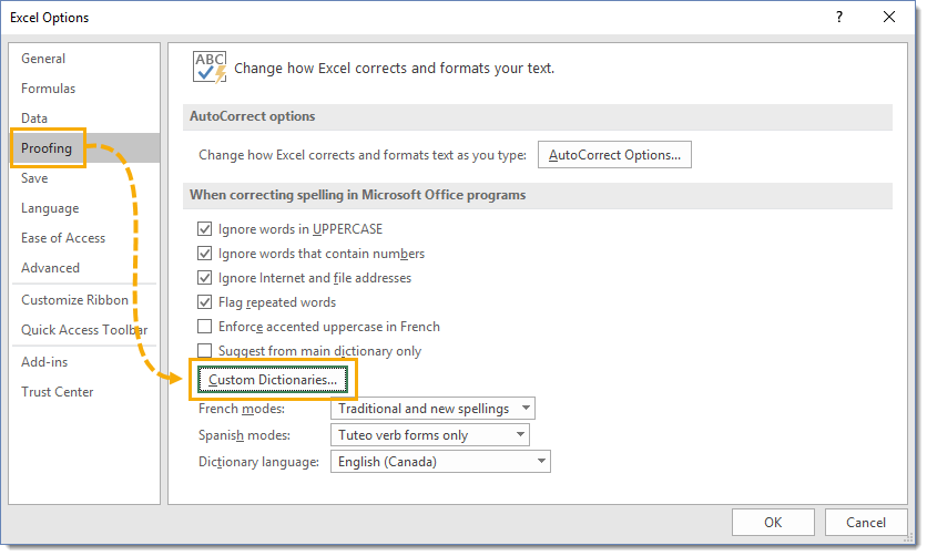
You can add your list to the dictionary in advance of them being flagged by spell check from the Excel Options. Go to the Proofing tab and press the Custom Dictionaries button.

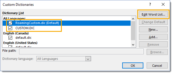
Select either the RoamingCustom.dic or CUSTOM.DIC dictionary lists and press the Edit Word List button to add any words.

Adding words one by one might not be ideal if you have a long list of words to add. You can search CUSTOM.DIC in your windows file explorer and edit the file directly to easily copy and paste your list with each word appearing on its own line.

Note that adding a word to the dictionary will add the word for all Excel workbooks opened on the same computer and in fact across all Microsoft Office applications.

List All Linked Files in a Workbook

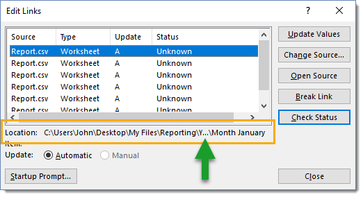
If your workbook contains links to external files you can see all of them listed by going to the Data tab and pressing the Edit Links button.

This will open the Edit Links dialog box where you can see all the links listed. The folder path will be displayed at the bottom for any link selected, but for long paths it will be truncated and you can’t copy the path from here.

There’s no obvious way to get a list of the file paths for any of the links.

We can use the LINKS() Excel 4.0 Macro for this! Excel 4.0 Macro’s are legacy functions from long ago before Excel VBA was introduced. They are still available, but can only be used with a defined name and not as a regular worksheet function.

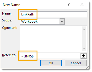
Go to the Formula tab and press the Define Name command found in the Defined Names section of the ribbon. Enter a name like LinkPath and add the formula =LINKS() in the refers to section and press OK.

Now add the formula =INDEX(LinkPath,ROW()) into cell A1 of any sheet and copy it down until all links are displayed.

Click and Drag to Cut and Paste

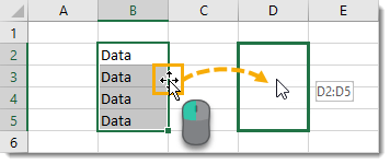
A quick way to cut and paste ranges of data is to click and drag.

Select the range and place the cursor over the green border. The cursor will change to a four way arrow and you can then left click and drag the range to a new location.

This is equivalent to cut and paste commands found in the Home tab.

Ctrl Click and Drag to Copy

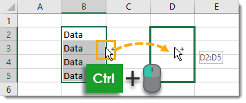
If you hold Ctrl while the cursor is on the range border, the cursor will show a small plus sign next to it. This means when you click and drag the range it will create a copy instead of moving the range.

This trick will work on many different Excel objects too, try this on tables, pivot tables, shapes and pictures to quickly make a copy.

Right Click and Drag for Advanced Features

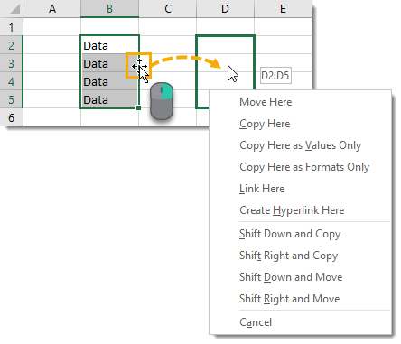
If you right click and drag a range instead of the usual left click, then you’ll able to do more than just cut and paste. A whole menu of advanced options is available.

• Move Here – This will cut and paste the selection to the new location.
• Copy Here – This will copy and paste the selection to the new location.
• Copy Here as Values Only – This will copy and paste only the values to the new location.
• Copy Here as Formats Only – This will copy and paste only the formatting to the new location.
• Link Here – This will create a simple cell reference formula to the old location in the new location.
• Create Hyperlink Here – This will create a hyperlinked cell reference to the old location in the new location.
• Shift Down and Copy – This will copy and paste the selection to the new location and shift down any previous data in the new location.
• Shift Right and Copy – This will copy and paste the selection to the new location and shift right any previous data in the new location.
• Shift Down and Move – This will cut and paste the selection to the new location and shift down any previous data in the new location.
• Shift Right and Move – This will cut and paste the selection to the new location and shift right any previous data in the new location
• Cancel – This will cancel the action.

Only Allow Unique Data in a Table Column

If you want to keep your data duplicate free, then you can use data validation rules to not allow any duplicate entries in your table of data.

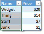
Select the column of data in your table where you don’t want duplicate values, then go to the Data tab and select Data Validation.

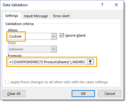
Then select a Custom criteria and enter the following formula into the formula section.

=COUNTIF(INDIRECT("Products[Name]"),INDIRECT("Products[@Name]"))=1

Here Products is the name of the table and Name is the name of the column. This will prevent anyone from entering duplicate values in this column of the table.

Make a Frequency Chart in Cell

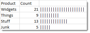
The REPT function takes a text string and repeats it a specified number of times. We can use this to create an in cell frequency chart. Use the formula =REPT("|",Count), where Count is the frequency count you want to graph.

Get the Column Width with a Formula

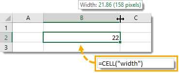
You can get the column width with a formula. Place the following formula in any column to return its width rounded to the nearest integer.

=CELL(“width”)

Unfortunately, there’s no row height equivalent.

Selecting and Deselecting Non-Continuous Ranges

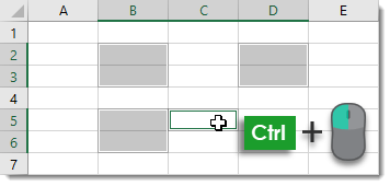
Hold Ctrl and left click on the cells to select non-continuous ranges. Hold Ctrl and left click on a selected cell to deselect it.

Use the Watch Window to Keep an Eye on Changing Values

If you’re making changes to a spreadsheet you can still keep an eye on cells that aren’t in the current viewable worksheet area by using the watch window.

This way you can more easily monitor if your changes are having the intended results. This is amazing when you need to track changes in far off cells on the same sheet or across multiple sheets.

Go to the Formula tab and select the Watch Window command from the ribbon.

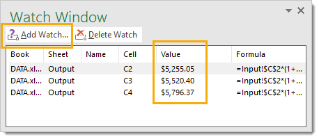
Select any cells you want to watch and then press the Add Watch button in the Watch Window. You’ll be able to see the current cell values listed and you can monitor unexpected changes.

The watch window may appear as a floating window, but you can click and drag it to either the left or right side to dock it to the workbook. This will also give you more vertical viewing area in the watch window to track more values at the same time.

Hide Zero Values

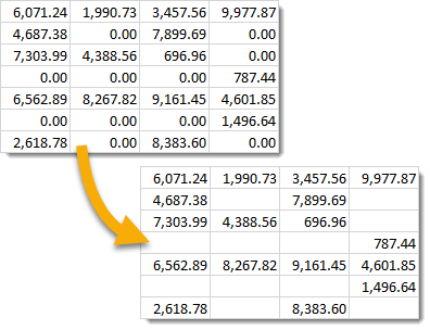
A lot of zeros in your data can be a distraction from the other non-zero values. You can change the settings so that the zeros don’t display in the worksheet. They will still be there, just not visible.

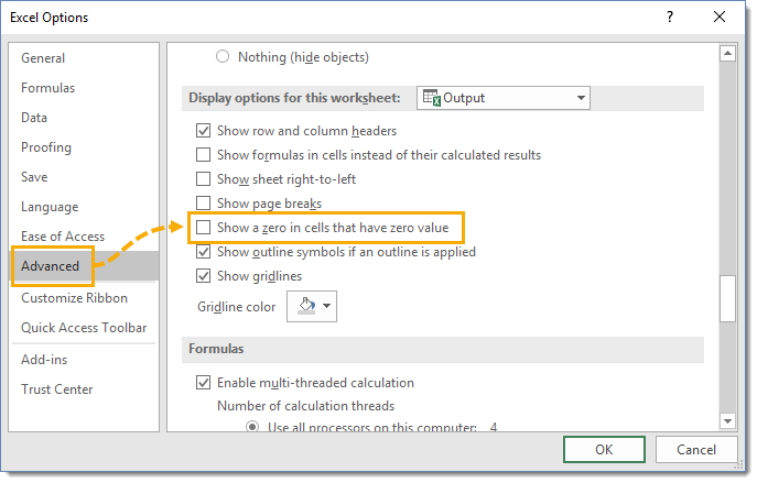
Open the Excel Options and go to the Advanced tab then scroll down to the Display options for this worksheet and uncheck the Show a zero in cells that have zero value.

This will get rid of all those pesky zeros. Careful though, this will affect the entire workbook. If you want to only hide zeros for a select range then use a custom format like #,##0.00;#,##0.00;;.

Change What the Mouse Wheel Does

If your mouse has a wheel on it, you can change the action if performs.

Normally it will scroll up or down a sheet but if you hold Ctrl while using the mouse wheel it will zoom in and out on the sheet.

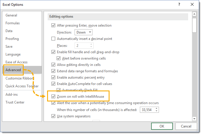
You can change this behavior permanently in the Excel Options. Go to the Advanced tab and check the Zoom on roll with IntelliMouse option. With this enabled, holding Ctrl while using the mouse wheel will revert to the vertical scrolling action.

Mouse Wheel Click to Scroll

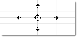
Some mouse wheels also act as a button you can press. If you have a mouse wheel and it’s also a button then pressing down on it will allow you to scroll around your worksheet with the cursor.

Click on the mouse wheel anywhere in the sheet and that will create the scroll anchor. Moving the cursor up, down, right or left in relation to the click point will scroll around the sheet in that direction.

The further you move the cursor away from the anchor point, the faster you will scroll.

Use Center Across Selection Instead of Merge and Center

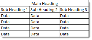
You may be tempted to create a heading for multiple columns using a merged and centered cell. Don’t do it! There are too many negative effects from merged cells.

Get the same visual effect using Center Across selection, without any of the negative consequences of merged cells.

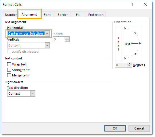
Select the cells where you want to create a main heading, then open the Format Cells dialog box by going to the Home tab and then clicking on the small icon in the lower right corner of the Number section or by using the Ctrl + 1 keyboard shortcut.

Under the Alignment tab select Center Across Selection and press the OK button. Before pressing Ok, you might also want to add an outer border to the selection to further create the look of a merged cell.

Unlimited Format Painter

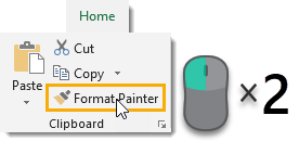
To use the format painter, you select the cells which you want to copy the format from and click on the Format Painter command found in the Home tab. This only gives you a one time use to paint the format.

If you double click on the Format Painter command, you get unlimited use. Just press Esc to exit format painting mode when you’re done.

Concatenate Text with an Ampersand

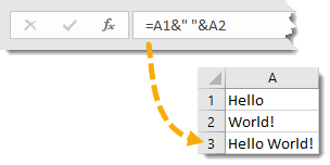
You may need to join separate text together. You can do this with the ampersand character &.

=A1&" "&A2

In this example we concatenate the text in two cells and add a space character between them.

Change the Colour of Any Sheet Tab

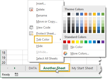
You can change the colour of any sheet tab. This is great for visually grouping similar sheets together in your workbook.

Right click on any sheet tab and select Tab Color from the menu. You can then choose from a variety of preset colours or create your own with the More Colors option.

You can change the colour of multiple sheets at the same time by holding Ctrl and selecting your sheets.