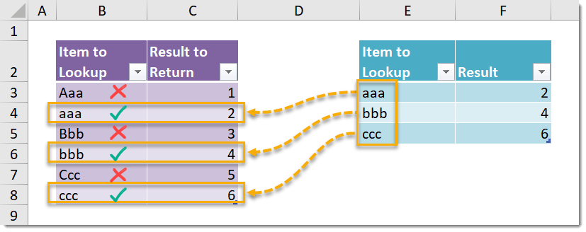
Example
Generic Formula
Note: This is an array formula. Do not type out the {} brackets. Hold Ctrl + Shift then press Enter while in Edit Mode to create an array formula.
- LookupItem – This is the value which you are looking up.
- LookupRange – This is the range of values in which you are trying to find the LookupItem.
- ResultsRange – This is the range of corresponding values to the LookupRange values. This range contains the values which you want to return as results from the lookup.
What It Does
This formula will perform a vertical case sensitive lookup in a given range of values and return a result from the corresponding cell in another range. The functionality of this formula is similar to the VLOOKUP function, however VLOOKUP does not differentiate between upper and lower case letters when looking for a match. To VLOOKUP “AAA” and “aaa” would be the same thing.
How It Works
This formula uses the EXACT function to create an array of Boolean values based on the LookupRange. This array will contain a TRUE value when the value in LookupRange is an exact match including case, and FALSE otherwise.
The formula then uses the MATCH function to find the position in the array of the first TRUE value. This position is used by the INDEX function to return the value in ResultsRange from the same position.
In our example, EXACT({“Aaa”;”aaa”;”Bbb”;”bbb”;”Ccc”;”ccc”},”aaa”) results in the following array of Boolean values.
This results in one TRUE value in the second position where we have an exact match to “aaa“.
MATCH(TRUE,{FALSE;TRUE;FALSE;FALSE;FALSE;FALSE},0) will then return 2 as a result because the first TRUE value is in the second position.
INDEX(ResultsRange,2,1) then returns 2 since the 2nd row and 1st column of our ResultsRange={1;2;3;4;5;6} contains a value of 2.
 👉 Find out more about our Advanced Formulas course!


0 Comments