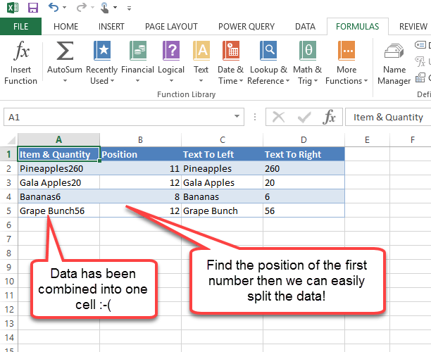
In this post we’re going to find out how to get the position of the first number within a text string. Let’s suppose we have stock level data for a grocery store and in our example someone has gone and put both the item and stock quantity in one cell making it difficult to use the data. How can we easily separate this data into two cells?
Copy and paste this table into cell A1 in Excel
| Item & Quantity | Position | Text To Left | Text To Right |
|---|---|---|---|
| Pineapples260 | =MIN(FIND({0,1,2,3,4,5,6,7,8,9},A2&”0123456789″)) | =LEFT(A2,B2-1) | =RIGHT(A2,LEN(A2)-B2+1) |
| Gala Apples20 | =MIN(FIND({0,1,2,3,4,5,6,7,8,9},A3&”0123456789″)) | =LEFT(A3,B3-1) | =RIGHT(A3,LEN(A3)-B3+1) |
| Bananas6 | =MIN(FIND({0,1,2,3,4,5,6,7,8,9},A4&”0123456789″)) | =LEFT(A4,B4-1) | =RIGHT(A4,LEN(A4)-B4+1) |
| Grape Bunch56 | =MIN(FIND({0,1,2,3,4,5,6,7,8,9},A5&”0123456789″)) | =LEFT(A5,B5-1) | =RIGHT(A5,LEN(A5)-B5+1) |
First to find the position of the first numeric character, we can use this formula.
=MIN(FIND({0,1,2,3,4,5,6,7,8,9},A2&"0123456789"))This will find the position of the first instance of one of the elements of the array {0,1,2,3,4,5,6,7,8,9} (i.e. the first number) within cell A2 (our text data). The &”0123456789″ part ensures the FIND function will at least find a number if A2 does not actually have a number in it and will allow the formula to calculate without resulting in a #VALUE error.
We can then use this position we have just calculated to return the text to the left (the item) and the text to the right (the quantity).
Text to the left can be found with this formula.
=LEFT(A2,B2-1)
Text to the right can be found with this formula.
=RIGHT(A2,LEN(A2)-B2+1)

 👉 Find out more about our Advanced Formulas course!


I tried cutting and pasting the example into Excel, and it didn’t work. I finally figured out the issue is that the font used here converted the quotation marks to characters that Excel didn’t recognize: ” ″. I changed them to ” and it worked fine.
Yes, unfortunately WordPress and Excel use a different quote character.
Works great!