Merged cells are one of the most popular options used by beginner spreadsheet users.

But they have a lot of drawbacks that make them a not so great option.

In this post, I’ll show you everything you need to know about merged cells including 8 ways to merge cells.

I’ll also tell you why you shouldn’t use them and a better alternative that will produce the same visual result.

What is a Merged Cell

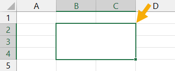
A merged cell in Excel combines two or more cells into one large cell. You can only merge contiguous cells that form a rectangular shape.

The above example shows a single merged cell resulting from merging 6 cells in the range B2:C4.

Why You Might Merge a Cell

Merging cells is a common technique used when a title or label is needed for a group of cells, rows or columns.

When you merge cells, only the value or formula in the top left cell of the range is preserved and displayed in the resulting merged cell. Any other values or formulas are discarded.

The above example shows two merged cells in B2:C2 and D2:F2 which indicates the category of information in the columns below. For example the First and Last name columns are organized with a Name merged cell.

Why is the Merge Command Disabled?

On occasion, you might find the Merge & Center command in Excel is greyed out and not available to use.

There are two reasons why the Merge & Center command can become unavailable.

• You are trying to merge cells inside an Excel table.
• You are trying to merge cells in a protected sheet.

Cells inside an Excel table can not be merged and there is no solution to enable this.

If most of the other commands in the ribbon are greyed out too, then it’s likely the sheet is protected. In order to access the Merge option, you will need to unprotect the worksheet.

This can be done by going to the Review tab and clicking the Unprotect Sheet command.

If the sheet has been protected with a password, then you will need to enter it in order to unprotect the sheet.

Now you should be able to merge cells inside the sheet.

Merged Cells Only Retain the Top Left Values

Warning before you start merging cells!

If the cells contain data or formulas, then you will lose anything not in the upper left cell.

A warning dialog box will appear telling you Merging cells only keeps the upper-left value and discards other values.

The above example shows the result of merging cells B2:C4 which contains text data. Only the data from cell B2 remains in the resulting merged cells.

If no data is present in the selected cells, then no warning will appear when trying to merge cells.

8 Ways to Merge a Cell

Merging cells is an easy task to perform and there are a variety of places this command can be found.

Merge Cells with the Merge & Center Command in the Home Tab

The easiest way to merge cells is using the command found in the Home tab.

1. Select the cells you want to merge together.
2. Go to the Home tab.
3. Click on the Merge & Center command found in the Alignment section.

Merge Cells with the Alt Hotkey Shortcut

There is an easy way to access the Home tab Merge and Center command using the Alt key.

Press Alt H M C in sequence on your keyboard to use the Merge & Center command.

Merge Cells with the Format Cells Dialog Box

Merging cells is also available from the Format Cells dialog box. This is the menu which contains all formatting options including merging cells.

You can open the Format Cells dialog box a few different ways.

• Go to the Home tab and click on the small launch icon in the lower right corner of the Alignment section.
• Use the Ctrl + 1 keyboard shortcut.
• Right click on the selected cells and choose Format Cells.

Go to the Alignment tab in the Format Cells menu then check the Merge cells option and press the OK button.

Merge Cells with the Quick Access Toolbar

If you use the Merge & Center command a lot, then it might make sense to add it to the Quick Access Toolbar so it’s always readily available to use.

Go to the Home tab and right click on the Merge & Center command then choose Add to Quick Access Toolbar from the options.

This will add the command to your QAT which is always available to use.

A nice bonus that comes with the quick access command is it gets its own hotkey shortcut based on its position in the QAT. When you press the Alt key, Excel will show you what key to press next in order to access the command.

In the above example, the Merge and Center command is the third command in the QAT so the hotkey shortcut is Alt 3.

Merge Cells with Copy and Paste

If you have a merged cell in your sheet already then you can copy and paste it to create more merged cells. This will produce merged cells with the exact same dimensions.

Copy a merged cell using Ctrl + C then paste it into a new location using Ctrl + V. Just make sure the paste area doesn’t overlap an existing merged cell.

Merge Cells with VBA

Sub MergeCells()
    Range("B2:C4").Merge
End Sub

The basic command for merging cells in VBA is quite simple. The above code will merge cells B2:C4.

Merge Cells with Office Scripts

function main(workbook: ExcelScript.Workbook) {
	let selectedSheet = workbook.getActiveWorksheet();
	selectedSheet.getRange("B2:C4").merge(false);
	selectedSheet.getRange("B2:C4").getFormat().setHorizontalAlignment(ExcelScript.HorizontalAlignment.center);
}

The above office script will merge and center the range B2:C4.

Merge Cells inside a PivotTable

We can’t make this change for the selected cells because it will affect a PivotTable. Use the field list to change the report. If you are trying to insert or delete cells, move the PivotTable and try again.

If you try to use the Merge and Center command inside a Pivot Table, you will be greeted with the above error message.

You can’t use the Merge & Center command inside a PivotTable, but there is a way to merge cells in the PivotTable options menu.

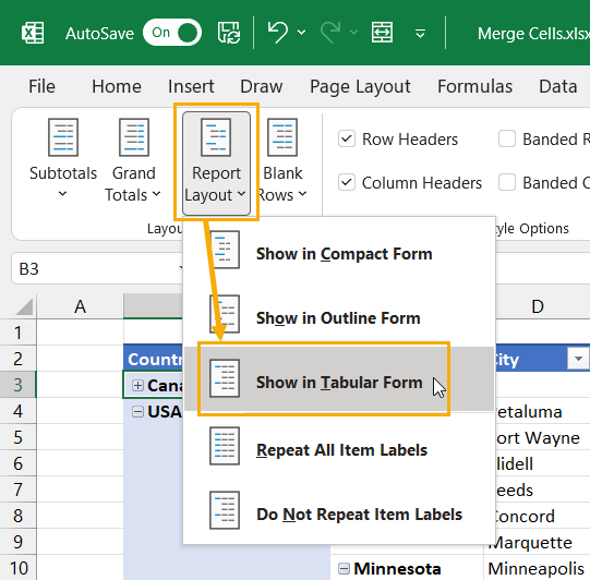
In order to avail of this option, you will first need to make sure your Pivot Table is in the tabular display mode.

1. Select a cell inside your PivotTable.
2. Go to the Design tab.
3. Click on Report Layout.
4. Choose Show in Tabular Form.

Your pivot table will now be in the tabular form where each field you add to the Rows area will be in its own column with data in a displayed in a single row.

Now you can enable the option to show merge cells inside the pivot table.

1. Select a cell inside your PivotTable.
2. Go to the PivotTable Analyze tab.
3. Click on Options.

This will open up the PivotTable Options menu.

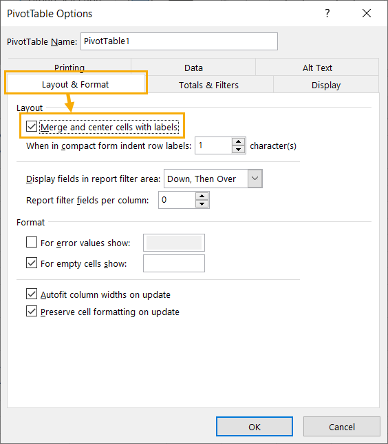
Enable the Merge and center cells with labels setting in the PivotTable Options menu.

1. Click on the Layout & Format tab.
2. Check the Merge and center cells with labels option.
3. Press the OK button.

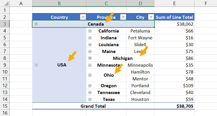
Now as you expand and collapse fields in your pivot table, fields will merge when they have a common label.

10 Ways to Unmerge a Cell

Unmerging a cell is also quick and easy. Most methods involve the same steps as used to merge the cell, but there are a few extra methods worth knowing.

Unmerge Cells with the Home Tab Command

This is the same process as merging cells from the Home tab command.

1. Select the merged cells to unmerge.
2. Go to the Home tab.
3. Click on the Merge & Center command.

Unmerge Cells with the Format Cells Menu

You can unmerge cells from the Format Cells dialog box as well.

Press Ctrl + 1 to open the Format Cells menu then go to the Alignment tab then uncheck the Merge cells option and press the OK button.

Unmerge Cells with the Alt Hot Key Shortcut

You can use the same Alt hot key combination to unmerge a merged cell. Select the merged cell you want to unmerge then press Alt H M C in sequence to unmerge the cells.

Unmerge Cells with Copy and Paste

You can copy the format from a regular single cell to unmerge merged cells.

Find a single cell and use Ctrl + C to copy it, then select the merged cells and press Ctrl + V to paste the cell.

You can use the Paste Special options to avoid overwriting any data when pasting. Press Ctrl + Alt + V then select the Formats option.

Unmerge Cells with the Quick Access Toolbar

This is a great option if you have already added the Merge & Center command to the quick access toolbar previously.

All you need to do is select the merged cells and click on the command or use the Alt hot key shortcut.

Unmerge Cells with the Clear Formats Command

Merged cells are a type of format, so it’s possible to unmerge cells by clearing the format from the cell.

1. Select the merged cell to unmerge.
2. Go to the Home tab.
3. Click on the right part of the Clear button found in the Editing section.
4. Select Clear Formats from the options.

Unmerge Cells with VBA

Sub UnMergeCells()
    Range("B2:C4").UnMerge
End Sub

Above is the basic command for unmerging cells in VBA. This will unmerge cells B2:C4.

Unmerge Cells with Office Scripts

Most methods of merging a cell can be performed again to unmerge cells like a toggle switch to merge or unmerge.

However the code in office scripts doesn’t work like this and instead, you will need to remove formatting to unmerge.

function main(workbook: ExcelScript.Workbook) {
	let selectedSheet = workbook.getActiveWorksheet();
	selectedSheet.getRange("B2:C4").clear(ExcelScript.ClearApplyTo.formats);
}

The above code will clear the format in cells B2:C4 and unmerge any merged cells it contains.

Unmerge Cells with the Accessibility Pane

Merged cells create problems for screen readers which is an accessibility issue. Because of this, they are flagged in the Accessibility window pane.

If you know the location of the merged cells, you can select them and go to the Review tab then click on the lower part of the Check Accessibility button and choose Unmerge Cells.

If you don’t know where all the merged cells are, you can open up the accessibility pane and it will show you where there are and you will be able to unmerge them one by one.

Go to the Review tab and click on the top part of the Check Accessibility command to launch the accessibility window pane.

This will show a Merged Cells section which you can expand to see all merged cells in the workbook. Click on the address and Excel will take you to that location.

Click on the downward chevron icon to the right of the address and the Unmerge option can be selected.

Unmerge Cells inside a PivotTable

To unmerge cells inside a pivot table, you just need to disable the setting in the pivot table options menu.

Now you can enable the option to show merge cells inside the pivot table.

1. Select a cell inside your PivotTable.
2. Go to the PivotTable Analyze tab.
3. Click on Options.
4. Click on the Layout & Format tab.
5. Uncheck the Merge and center cells with labels option.
6. Press the OK button.

Merge Multiple Ranges in One Step

In Excel, you can select multiple non-continuous ranges in a sheet by holding the Ctrl key. A nice consequence of this is you can convert these multiple ranges into merged cells in one step.

Hold the Ctrl key while selecting multiple ranges with the mouse. When you’re finished selecting the ranges you can release the Ctrl key and then go to the Home tab and click on the Merge & Center command.

Each range will become its own merged cell.

Combine Data Before Merging Cells

Before you merge any cells which contain data, it’s advised to combine the data since only the data in the top left cell is preserved when merging cells.

There are a variety of ways to do this, but using the TEXTJOIN function is among the easiest and most flexible as it will allow you to separate each cell’s data using a delimiter if needed.

= TEXTJOIN ( ", ", TRUE, B2:C4 )

The above formula will join all the text in range B2:C4 going from left to right and then top to bottom. Text in each cell is separated with a comma and space.

Once you have the formula result, you can copy and paste it as a value so that the data is retained when you merge the cells.

How to Get Data from Merged Cells in Excel

A common misconception is that each cell of in the merged range contains the data entered inside.

In fact, only the top left cell will contain any data.

In the above example, the formula references the top left value in the merged range. The result returned is what is seen in the merged range.

In this example, the formula references a cell that is not the top left most cell in the merged range. The result is 0 because this cell is empty and contains no value.

In order to extract data from a merged range, you will always need to reference the top left most cell of the range. Fortunately, Excel automatically does this for you when you select the merged cell in a formula.

How to Find Merged Cells in a Workbook

If you create a bunch of merged cells, you might need to find them all later. Thankfully it’s not a painful process.

This can be done using the Find & Select command.

Go to the Home tab and click on the Find & Select button found in the Editing section, then choose the Find option. This will open the Find and Replace menu

You can also use the Ctrl + F keyboard shortcut.

You don’t need to enter any text to find, you can use this menu to find cells formatted as merged cells.

1. Click on the Format button to open the Find Format menu.
2. Go to the Alignment tab.
3. Check the Merge cells option.
4. Press the OK button in the Find Format menu.
5. Press the Find All or Find Next button in the Find and Replace menu.

Unmerge All Merged Cells

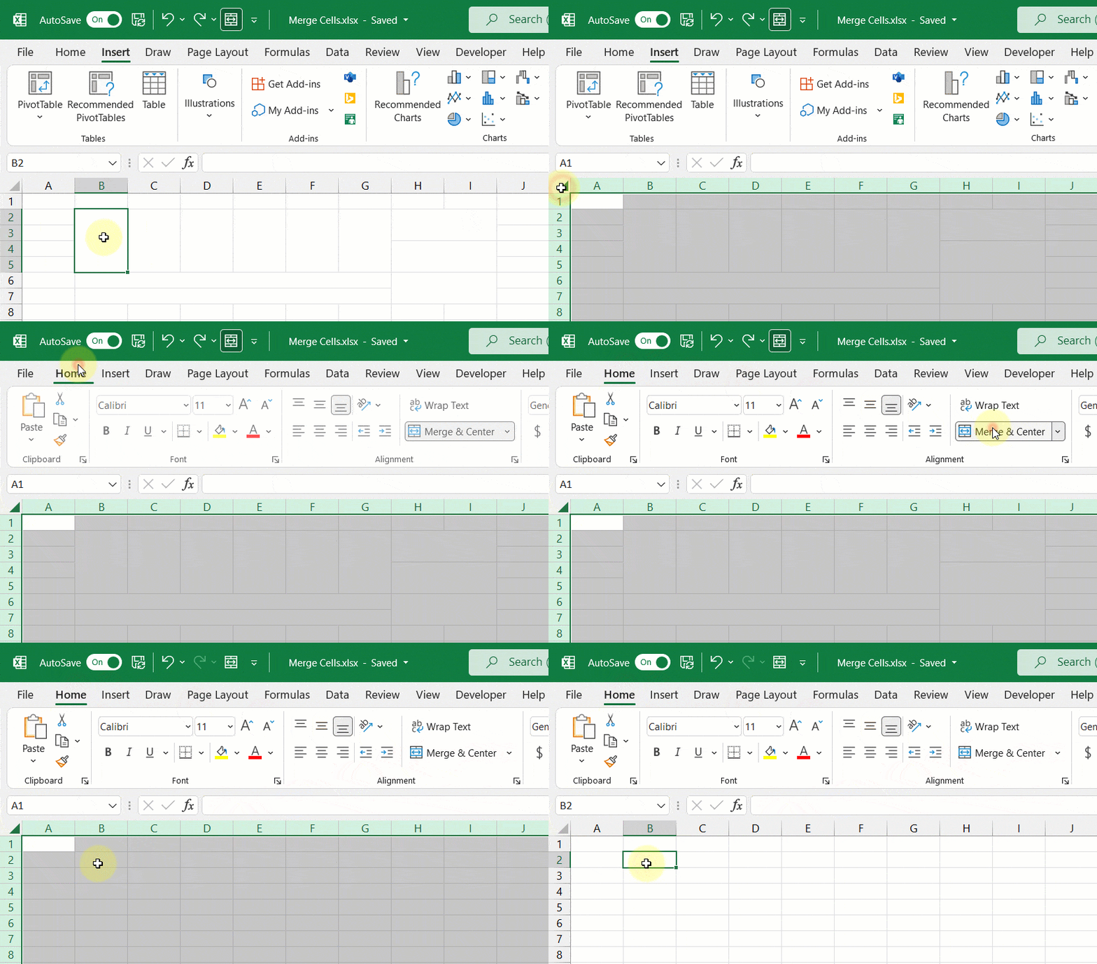
Fortunately, unmerging all merged cells in a sheet is very easy.

1. Select the entire sheet. You can do this two ways.
   • Click on the select all button where the column headings meet the row headings.
   • Press Ctrl + A on your keyboard.
2. Go to the Home tab.
3. Press the Merge & Center command.

This will unmerge all the merged cells and leave all the other cells unaffected.

Why You Shouldn’t Merge Cells

There are a lot of reasons why you shouldn’t merge cells.

• You can’t sort data with merged cells.
• You can’t filter data with merged cells.
• You can’t copy and paste values into merged cells.
• It will create accessibility problems for screen readers by changing the order in which text should be read.

This isn’t an exhaustive list, there are likely many more you will come across should you choose to merge cells.

Alternative to Merging a Cell

Good news!

There is a much better alternative than merging cells.

This alternative has none of the negative features that come with merging cells but will still allow you to achieve the same visual look of a merged cell.

It will allow you to display text centered across a range of cells without merging the cells.

Unfortunately, this technique will only work horizontally with one row of cells. There is no option to do something similar with a vertical range of cells.

Select the horizontal range of cells that you would like to center your text across. The first cell should contain the text which is to be centered while the remaining cells should be empty.

This example shows text in cell B2 and the range B2:C2 is selected as the range to center across.

Go to the Home tab and click on the small launch icon in the lower right corner of the Alignment section. This will open up the Format Cells dialog box with the Alignment tab active.

You can also press Ctrl + 1 to open the Format Cells dialog box and navigate to the Alignment tab.

Select Center Across Selection from the Horizontal dropdown options in the Text alignment section.

The text will now appear as though it occupies all cells but it will only exist in the first cell of the centering selection and each cell is still separate.

Pros

• The text appears centered across the selected range similar to a merged cell.
• No negative effects from merged cells.
• Can be used inside an Excel table.

Cons

• Can not center across a vertical range of cells.

Conclusions

There are lots of ways to merge cells in Excel. You can also easily unmerge cells too if you need to.

There are many things to consider when merging cells in Excel.

As you have seen, there are lots of pitfalls to merged cells that you should consider before implementing them in your workbooks.

Do you have a favorite merge method or warning about the dangers of merged cells that are not listed in the post? Let me know about it in the comments.