Duplicate values in your data can be a big problem! It can lead to substantial errors and over estimate your results.

But finding and removing them from your data is actually quite easy in Excel.

In this tutorial, we are going to look at 7 different methods to locate and remove duplicate values from your data.

Video Tutorial

What Is A Duplicate Value?

Duplicate values happen when the same value or set of values appear in your data.

For a given set of data you can define duplicates in many different ways.

In the above example, there is a simple set of data with 3 columns for the Make, Model and Year for a list of cars.

1. The first image highlights all the duplicates based only on the Make of the car.
2. The second image highlights all the duplicates based on the Make and Model of the car. This results in one less duplicate.
3. The second image highlights all the duplicates based on all columns in the table. This results in even less values being considered duplicates.

The results from duplicates based on a single column vs the entire table can be very different. You should always be aware which version you want and what Excel is doing.

Find And Remove Duplicate Values With The Remove Duplicates Command

Removing duplicate values in data is a very common task. It’s so common, there’s a dedicated command to do it in the ribbon.

Select a cell inside the data which you want to remove duplicates from and go to the Data tab and click on the Remove Duplicates command.

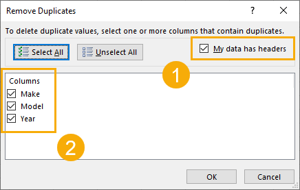
Excel will then select the entire set of data and open up the Remove Duplicates window.

1. You then need to tell Excel if the data contains column headers in the first row. If this is checked, then the first row of data will be excluded when finding and removing duplicate values.
2. You can then select which columns to use to determine duplicates. There are also handy Select All and Unselect All buttons above you can use if you’ve got a long list of columns in your data.

When you press OK, Excel will then remove all the duplicate values it finds and give you a summary count of how many values were removed and how many values remain.

This command will alter your data so it’s best to perform the command on a copy of your data to retain the original data intact.

Find And Remove Duplicate Values With Advanced Filters

There is also another way to get rid of any duplicate values in your data from the ribbon. This is possible from the advanced filters.

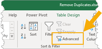
Select a cell inside the data and go to the Data tab and click on the Advanced filter command.

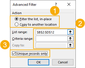
This will open up the Advanced Filter window.

1. You can choose to either to Filter the list in place or Copy to another location. Filtering the list in place will hide rows containing any duplicates while copying to another location will create a copy of the data.
2. Excel will guess the range of data, but you can adjust it in the List range. The Criteria range can be left blank and the Copy to field will need to be filled if the Copy to another location option was chosen.
3. Check the box for Unique records only.

Press OK and you will eliminate the duplicate values.

Advanced filters can be a handy option for getting rid of your duplicate values and creating a copy of your data at the same time. But advanced filters will only be able to perform this on the entire table.

Find And Remove Duplicate Values With A Pivot Table

Pivot tables are just for analyzing your data, right?

You can actually use them to remove duplicate data as well!

You won’t actually be removing duplicate values from your data with this method, you will be using a pivot table to display only the unique values from the data set.

First, create a pivot table based on your data. Select a cell inside your data or the entire range of data ➜ go to the Insert tab ➜ select PivotTable ➜ press OK in the Create PivotTable dialog box.

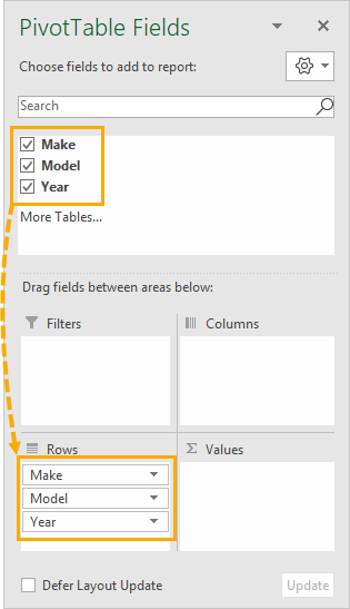
With the new blank pivot table add all fields into the Rows area of the pivot table.

You will then need to change the layout of the resulting pivot table so it’s in a tabular format. With the pivot table selected, go to the Design tab and select Report Layout. There are two options you will need to change here.

1. Select the Show in Tabular Form option.
2. Select the Repeat All Item Labels option.

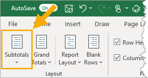
You will also need to remove any subtotals from the pivot table. Go to the Design tab ➜ select Subtotals ➜ select Do Not Show Subtotals.

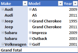
You now have a pivot table that mimics a tabular set of data!

Pivot tables only list unique values for items in the Rows area, so this pivot table will automatically remove any duplicates in your data.

Find And Remove Duplicate Values With Power Query

Power Query is all about data transformation, so you can be sure it has the ability to find and remove duplicate values.

Select the table of values which you want to remove duplicates from ➜ go to the Data tab ➜ choose a From Table/Range query.

Remove Duplicates Based On One Or More Columns

With Power Query, you can remove duplicates based on one or more columns in the table.

You need to select which columns to remove duplicates based on. You can hold Ctrl to select multiple columns.

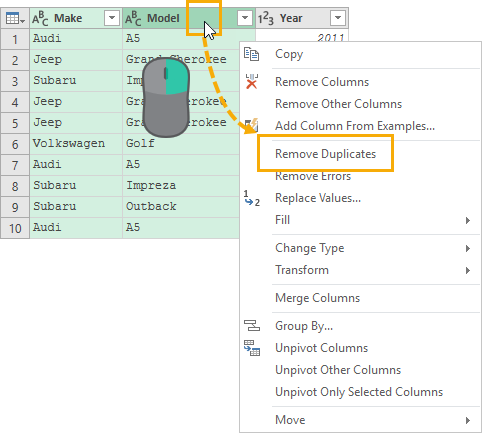
Right click on the selected column heading and choose Remove Duplicates from the menu.

You can also access this command from the Home tab ➜ Remove Rows ➜ Remove Duplicates.

= Table.Distinct(#"Previous Step", {"Make", "Model"})

If you look at the formula that’s created, it is using the Table.Distinct function with the second parameter referencing which columns to use.

Remove Duplicates Based On The Entire Table

To remove duplicates based on the entire table, you could select all the columns in the table then remove duplicates. But there is a faster method that doesn’t require selecting all the columns.

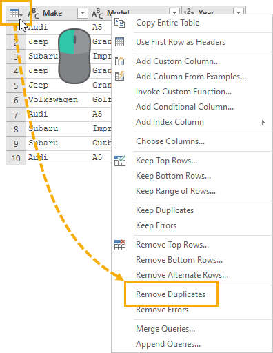
There is a button in the top left corner of the data preview with a selection of commands that can be applied to the entire table.

Click on the table button in the top left corner ➜ then choose Remove Duplicates.

= Table.Distinct(#"Previous Step")

If you look at the formula that’s created, it uses the same Table.Distinct function with no second parameter. Without the second parameter, the function will act on the whole table.

Keep Duplicates Based On A Single Column Or On The Entire Table

In Power Query, there are also commands for keeping duplicates for selected columns or for the entire table.

Follow the same steps as removing duplicates, but use the Keep Rows ➜ Keep Duplicates command instead. This will show you all the data that has a duplicate value.

Find And Remove Duplicate Values Using A Formula

You can use a formula to help you find duplicate values in your data.

First you will need to add a helper column that combines the data from any columns which you want to base your duplicate definition on.

= [@Make] & [@Model] & [@Year]

The above formula will concatenate all three columns into a single column. It uses the ampersand operator to join each column.

= TEXTJOIN("", FALSE , CarList[@[Make]:[Year]])

If you have a long list of columns to combine, you can use the above formula instead. This way you can simply reference all the columns as a single range.

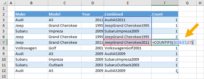
You will then need to add another column to count the duplicate values. This will be used later to filter out rows of data that appear more than once.

= COUNTIFS($E$3:E3, E3)

Copy the above formula down the column and it will count the number of times the current value appears in the list of values above.

If the count is 1 then it’s the first time the value is appearing in the data and you will keep this in your set of unique values. If the count is 2 or more then the value has already appeared in the data and it is a duplicate value which can be removed.

Add filters to your data list.

• Go to the Data tab and select the Filter command.
• Use the keyboard shortcut Ctrl + Shift + L.

Now you can filter on the Count column. Filtering on 1 will produce all the unique values and remove any duplicates.

You can then select the visible cells from the resulting filter to copy and paste elsewhere. Use the keyboard shortcut Alt + ; to select only the visible cells.

Find And Remove Duplicate Values With Conditional Formatting

With conditional formatting, there’s a way to highlight duplicate values in your data.

Just like the formula method, you need to add a helper column that combines the data from columns. The conditional formatting doesn’t work with data across rows, so you’ll need this combined column if you want to detect duplicates based on more than one column.

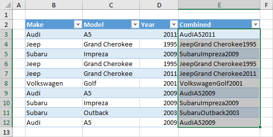
Then you need to select the column of combined data.

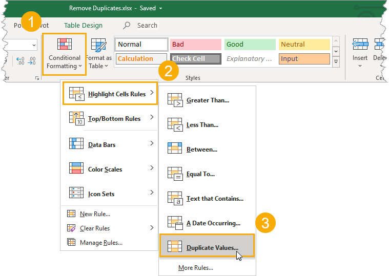
To create the conditional formatting, go to the Home tab ➜ select Conditional Formatting ➜ Highlight Cells Rules ➜ Duplicate Values.

This will open up the conditional formatting Duplicate Values window.

1. You can select to either highlight Duplicate or Unique values.
2. You can also choose from a selection of predefined cell formats to highlight the values or create your own custom format.

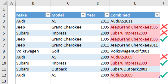
Warning: The previous methods to find and remove duplicates considers the first occurrence of a value as a duplicate and will leave it intact. However, this method will highlight the first occurrence and will not make any distinction.

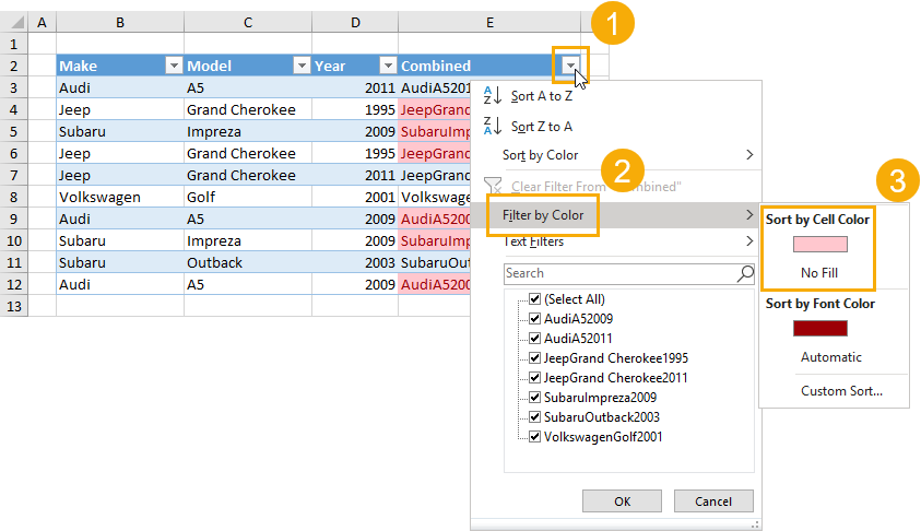
With the values highlighted, you can now filter on either the duplicate or unique values with the filter by color option. Make sure to add filters to your data. Go to the Data tab and select the Filter command or use the keyboard shortcut Ctrl + Shift + L.

1. Click on the filter toggle.
2. Select Filter by Color in the menu.
3. Filter on the color used in the conditional formatting to select duplicate values or filter on No Fill to select unique values.

You can then select just the visible cells with the keyboard shortcut Alt + ;.

Find And Remove Duplicate Values Using VBA

There is a built in command in VBA for removing duplicates within list objects.

Sub RemoveDuplicates() Dim DuplicateValues As Range Set DuplicateValues = ActiveSheet.ListObjects("CarList").Range DuplicateValues.RemoveDuplicates Columns:=Array(1, 2, 3), Header:=xlYes End Sub

The above procedure will remove duplicates from an Excel table named CarList.

Columns:=Array(1, 2, 3)

The above part of the procedure will set which columns to base duplicate detection on. In this case it will be on the entire table since all three columns are listed.

Header:=xlYes

The above part of the procedure tells Excel the first row in our list contains column headings.

You will want to create a copy of your data before running this VBA code, as it can’t be undone after the code runs.

Conclusions

Duplicate values in your data can be a big obstacle to a clean data set.

Thankfully, there are many options in Excel to easily remove those pesky duplicate values.

So, what’s your go to method to remove duplicates?