If you’ve ever learnt some statistics, then you’ve probably come across the correlation coefficient.

But can you calculate this in Excel?

Yes, you can!

Excel can be a great tool for a statistician when you know how to use it.

In this post, I’ll show you 3 ways to calculate the correlation coefficient in Excel.

Video Tutorial

What is a Correlation Coeffecient?

The correlation coefficient is also known as the Pearson Correlation Coefficient and it is a measurement of how related two variables are.

The calculation can have a value between 0 and 1.

A value of 0 indicates the two variables are highly unrelated and a value of 1 indicates they are highly related.

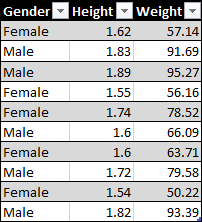
For example, you might have data on height (meters) and weight (kilograms) for a sample of people and want to know if these two variables are related.

Intuitively, you would think a person’s height and weight are related, but the correlation coefficient will show you mathematically how related or unrelated these are.

Correlation Coefficient Formula

The correlation coefficient r can be calculated with the above formula where x and y are the variables which you want to test for correlation.

In this example, the x variable is the height and the y variable is the weight. r is then the correlation between height and weight.

Calculating the Correlation Coefficient from the Definition

Let’s see how we can calculate this in Excel based on the above definition.

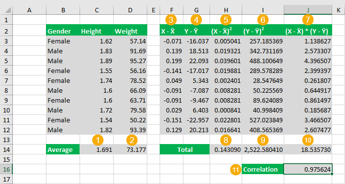
There are quite a few steps involved to calculate the correlation coefficient from scratch.

1. Calculate the average height.

   = AVERAGE ( C3:C12 )

2. Calculate the average weight.

   = AVERAGE ( D3:D12 )

3. Calculate the difference between the height and average height for each data point. This formula will need to be copied down for each row.

   = C3 - $C$14

4. Calculate the difference between the weight and average weight for each data point. This formula will need to be copied down for each row.

   = D3 - $D$14

5. Calculate the square of the difference from step 3 for each row.

   = POWER ( F3, 2 )

6. Calculate the square of the difference from step 4 for each row.

   = POWER ( G3, 2 )

7. Calculate the product of differences from step 3 and 4 for each row.

   = F3 * G3

8. Calculate the sum of the squared differences from step 5.

   = SUM ( H3:H12 )

9. Calculate the sum of the squared differences from step 6.

   = SUM ( I3:I12 )

10. Calculate the sum of the product of differences from step 7.

    = SUM ( J3:J12 )

11. Calculate the correlation with the following formula.

    = J14 / ( SQRT ( H14 ) * SQRT ( I14 ) )

It’s quite an involved calculation with a lot of intermediate steps.

Thankfully Excel has a built in function for getting the correlation which makes the calculation much more simple.

CORREL Function

This is a function specifically for calculating the Pearson correlation coefficient in Excel.

It’s very easy to use. It takes two ranges of values as the only two arguments.

= CORREL ( Variable1, Variable2 )

• Variable1 and Variable2 are the two variables which you want to calculate the Pearson Correlation Coefficient between.
• These are required inputs and must be a single column or single row array of numbers. Variable1 and Variable2 must also have the same dimension.

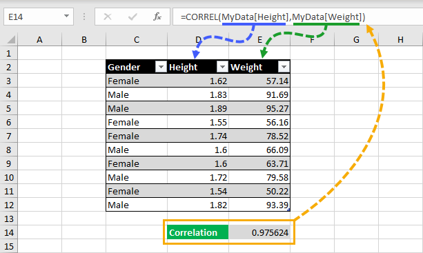
= CORREL ( Height, Weight )

The above formula is what you would need to calculate the correlation between height and weight.

Wow, so much easier than calculating it from scratch!

This method is also dynamic. If your data changes, the correlation calculation will update to reflect the new data.

Statistical Tools

Excel comes with a powerful statistical tools add-in, but you need to enable it to use it first and it’s quite hidden.

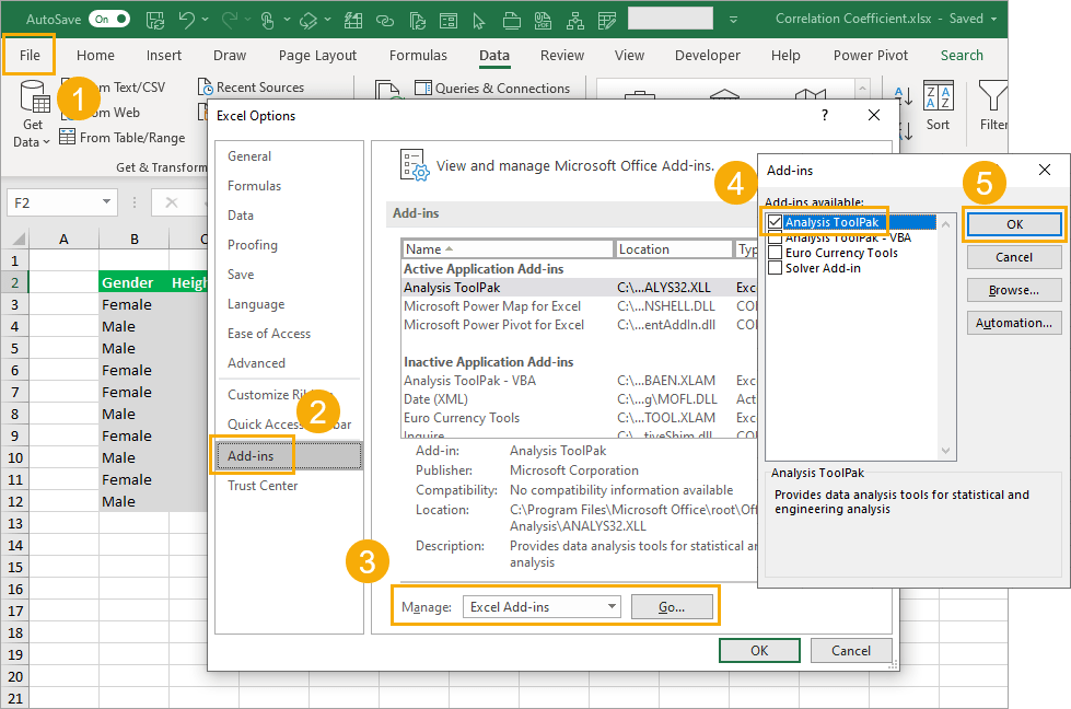
To enable the Analysis ToolPak:

1. Go to the File tab and then choose Options.
2. Go to the Add-ins tab in the Excel Options.
3. Choose Excel Add-ins from the drop-down list and press the Go button.
4. Check the Analysis ToolPak option from the available add-ins.
5. Press the OK button.

You will now have a Data Analysis command available in the Data tab and you can click on this to open up the Analysis ToolPak.

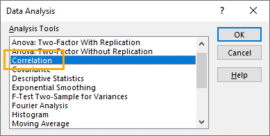
This will open up the Data Analysis menu and you can then select Correlation from the options and press the OK button.

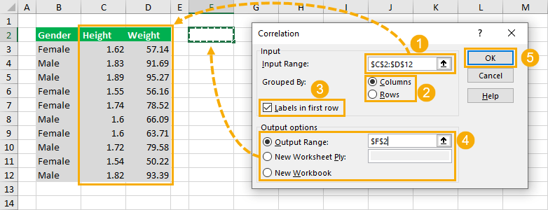
This will open up the Data Analysis Correlation menu.

1. Supply the Input Range for the correlation calculation. This should be a range with numerical values organized into columns or rows.
2. Select the Group By option of Columns or Rows. This example has the data organized by columns as values for height are all in one column and values for weight are in a separate column.
3. Select whether or not your input range has Labels in the first row. These labels are used later in the output so it’s best to select an input range that includes the labels.
4. Select where to place the output in the Output options. You can choose from a location in the current sheet, a location in a new sheet, or a new workbook.
5. Press the OK button create the calculation.

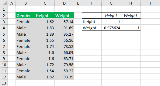
This will output a correlation matrix.

This means if you have more than two columns of variable, the matrix will contain the correlation coefficient for all combinations of variables.

The drawback of this method is the output is static. If your data changes, you will need to rerun the data analysis to update the correlation matrix.

Conclusions

Correlation is a very useful statistic to determine if your data is related.

The mathematical formula can be intimidating though, especially when trying to calculate it in Excel.

Thankfully there are a few easy ways to implement this calculation in Excel.