Strikethrough formatting is a seldom used but extremely useful font formatting in most applications.

Strikethrough font can be a good great way to visually indicate something has been deleted, removed or is no longer relevant without actually removing it from your text.

This formatting option is also available in Excel, but unfortunately it’s not available directly from the ribbon commands. However it can be accessed in quite a few ways.

This post will show you all the ways you can add strikethrough font to your Excel workbooks.

Add Strikethrough Format from the Home Tab

Strikethrough formatting can be added to any cell or range of cells using the Format Cells dialog box and you can open this menu from the Home tab.

To add strikethrough formatting.

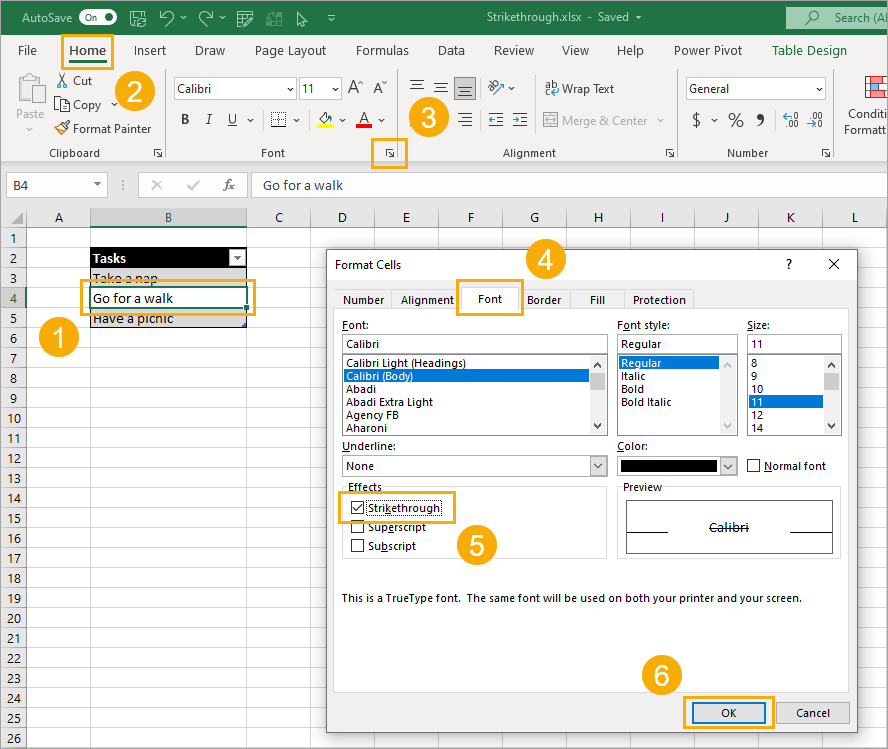
1. Select the cell or range of cells to which you would like to add the strikethrough formatting.
2. Go to the Home tab.
3. Click on the launch button in the lower right corner of the Font section. This will open up the Format Cells dialog box.
4. Go to the Font tab.
5. Check the option for Strikethrough.
6. Press the OK button.

Your text will now have a strikethrough format!

Other Ways to Open Format Cells and Add Strikethrough

Opening the Format Cells menu from the Home tab can be pretty slow. Thankfully there are quite a few other ways to open this menu that don’t take as many clicks.

Format Cells with Right Click Menu

You can open this menu from anywhere in any sheet by a right click. This will open up a large menu of actions and towards the bottom you will find Format Cells.

From here you’ll be able to add strikethrough just like before.

Format Cells Keyboard Shortcut

If you prefer to use the keyboard, there is a shortcut every Excel user should know for opening the Format Cells dialog box.

Press Ctrl + 1 and this will open up the Format Cells menu and you can then apply strikethrough format.

Format Cells Font Keyboard Shortcuts

The Format Cells dialog has a memory, so if you’ve used the Font tab the last time you had it open then it will open with the Font tab in focus.

If you want to guarantee the Format Cells dialog opens on the Font tab, there is are two keyboard shortcuts that will do this.

This first of these shortcuts is Ctrl + Shift + F. This is easy to remember since F stands for Font.

The other shortcut is Ctrl + Shift + P.

Both shortcuts will open up a limited version of the Format Cells dialog box which only contains the Font tab. This means it’s not a great choice is you also want to apply other formatting at the same time as you apply the strikethrough format.

Strikethrough Format Keyboard Shortcut

The previous keyboard shortcuts are great for accessing all sorts of formatting, but there is a more direct one available to apply strikethrough without opening the Format Cells menu.

Select any cells to which you want to apply strikethrough format and press Ctrl + 5.

This will instantly apply the strikethrough format without any format menu needed.

If you use strikethrough a lot, then this is one you need to remember. It’s not that hard either when you realize 5 looks like an S, and S stands for Strikethrough.

Add Strikethrough with the Quick Access Toolbar

For the people who prefer using the mouse over keyboard shortcuts, there is a quicker way than using the Format Cells menu.

You can add this to the Quick Action Toolbar so it’s always a one click process to add strikethrough.

Right click anywhere in the quick access toolbar and select Customize Quick Access Toolbar.

In the Excel Options menu.

1. Select All Commands from the drop down.
2. Scroll down and select Strikethrough in the list of available commands.
3. Press the Add button to add this into your QAT.
4. Press the OK button to close the menu.

Now this command is prominently available anytime you need to apply strikethrough format.

Apply Partial Strikethrough Format to a Cell

Up to now, you have learnt how to apply strikethrough format to all the contents of a cell or range of cells.

You can also use any of these techniques to apply a the formatting to only a part of the cell contents. This way you can strikethrough just a couple a words within a sentence in a cell.

Select a cell then select part of the text in the formal bar to which you want to apply the strikethrough format.

With the text selected inside the formula bar, you can now use any of the above methods to apply the strikethrough to just the selected part.

Remove Strikethrough Format

Removing any strikethrough format in your text is just as easy as applying it.

Select any cells which you want to remove the formatting from and you can use any of these methods.

• Uncheck the Strikethrough option in the Format Cells menu.
• Press the Ctrl + 5 keyboard shortcut.
• Press the Strikethrough command from the quick access toolbar.

Add Strikethrough Conditional Formatting

A great use for strikethrough formatting is to use it in your Excel checklists.

For this you can use conditional formatting to apply strikethrough to items on your checklist when you set a status to Done. This can feel very satisfying!

To set this up.

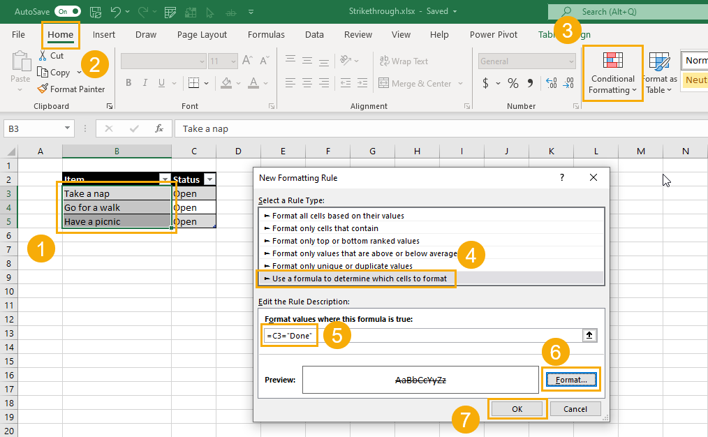
1. Select the column of cells to which you want to add strikethrough.
2. Go to the Home tab.
3. Select Conditional Formatting from the ribbon and select New Rule from the options.
4. Select Use a formula to determine which cells to format.
5. Enter =C3="Done" in the formula where C3 is the first cell in the Status column and Done is the value which you want to trigger the formatting.
6. Press the Format button and choose the Strikethrough option.
7. Press the OK button.

Now your task list items will automatically get a strikethrough formatting to indicate they have been completed whenever you set the status to done.

Conclusions

Even though this useful formatting option isn’t directly available in the ribbon, there are still quite a few ways to use it.

Whether you use the mouse or keyboard there is an option for you.

Do you know any other methods? Let me know in the comments!