Excel has some great features available in paste special, but where Excel is lacking is the ability to do any sort of cut and paste special. One feature I’ve wanted is the ability to cut and paste transpose this can be handy as using copy and paste transpose won’t always result in formulas keeping the correct references. In this post we’ll explore a work around method to get the same results as a cut and paste transpose would give (if it existed).
Step 1: Replace Any Formula With Text
Replace any formula with text in the range which you want to transpose.
- Highlight the range you want to transpose.
- Go to the Home tab in the ribbon.
- Under the Editing section press the Find & Select button.
- Select Replace from the menu. Alternatively, you can use the Ctrl + H keyboard shortcut to open the Find and Replace window.
- In the Find what box type in = and in the Replace with box type in #=. This will turn any formula into a text string. I like to use # as it’s a character that’s unlikely to appear in any of the formula’s but you can use any text in front of the equal sign as long as it’s not in any of your formulas.
- Press the Replace All button.
- Press the OK button in the pop up. It should say we made 6 replacements as there were 6 formula’s in our range.
- Press the Close button.
Step 2: Copy And Paste Transpose
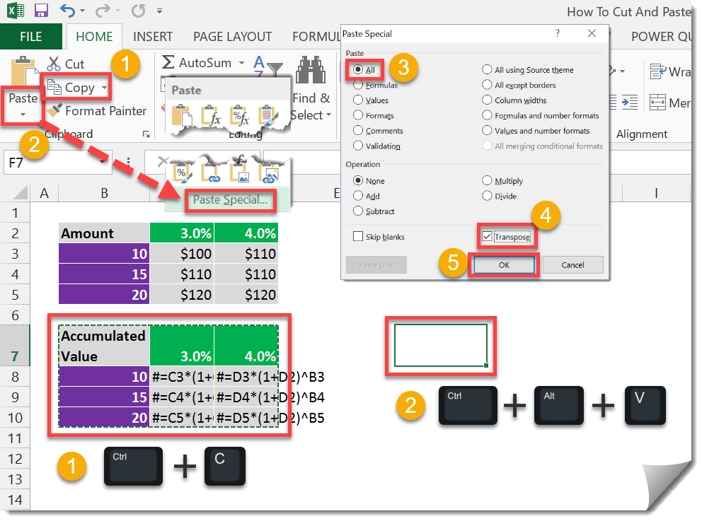
Now we can transpose our selection with copy and paste special.
- Highlight and copy the range which you want to transpose . You can either use the Ctrl + C keyboard shortcut or the Copy button in the Home tab of the ribbon.
- Select an empty cell where you want the transposed version and paste special. You can either use the Ctrl + Alt + V keyboard shortcut or the Paste button in the Home tab of the ribbon.
- Select the All radio button under the Paste options.
- Check the Transpose box.
- Press the OK button.
Step 3: Change The Transpose Range Back To Formula
Now we just need to change the text in the transposed version back to formulas.
- Select the transposed range.
- Open the Find and Replace window with the Ctrl + H keyboard shortcut or from the Home tab in the ribbon.
- In the Find what box type in #= and in the Replace with box type in =.
- Press the Replace All button. Press the OK button in the pop up that follows, again it should say we made 6 replacements as there were 6 formula’s in our range.
- Press the Close button.
Now we have a transposed version of the original range and all the formula’s have maintained their original references.


 👉 Find out more about our Advanced Formulas course!


Dear Sir/Madam – Your method show here is built and dangerously unreliable assumptions. Your method assumes the formulas in the copy/paste group do NOT refer to each other. If a single cells in the copy range references another cell in the copy range, it will point to the WRONG cells after the transformation (unless the cell it points to is on the exact diagonal of the matrix)! You really need to correct that ASAP. I hope nobody has used your advice for anything important. For example, if an engineer uses this method while designing safety features in an elevator YOU will be riding in, it could be your last ride. :-b
I wish I had spell checked that. I rewrote it and that always creates problems! ?
Good point! I never considered that case when I thought of the solution as my use case didn’t have internal linking.
I’d hope people check their work independently.
This works great if you don’t have any cells referencing the range being transposed. But as this isn’t a true cut action, any references to the original range won’t be redirected to the new transposed cells. This is what I have been trying to figure out and can’t find any work-arounds online anywhere. The range I need transposed serves as a data entry point that feeds into multiple other sheets, so updating the formulas referencing the range isn’t practicable.
Yes, it only takes care of references in the cells you are cutting.
Maybe try power query to transpose the data from the data entry area to the format you require.