This post is going to show you all the different methods you can insert a pivot table in Microsoft Excel.

Pivot tables are the best way to quickly summarize and analyze large sets of data in Excel.

They are easy to use and you can have a summarized report for your dataset in a few quick clicks.

There are a lot of entry points for pivot tables, and they are all worth knowing.

Get your copy of the example workbook to follow along.

Create an Excel Table for Your Dataset

The first thing you need to know about pivot tables, is they work best when the source data is inside an Excel Table.

Tables are structured objects that contain data. When you have a tabular dataset, you should put it in a Table.

Here is an example dataset of product orders.

Before you put your data inside a table, you will need to make sure it is in the correct tabular format.

1. The first row should contain column headings. This should be a short text describing the data contained below.
2. There should be no blank column headings. Every column of data should have a name.
3. There should be no blank columns or blank rows.
4. There should be no subtotals or grand totals within the data.
5. One row should represent exactly one record of data. In the example data, 1 row equates to the sale of one product in a customer’s order.
6. One column should contain exactly 1 type of data. in the example data, the Item column only contains information on the name of the product.

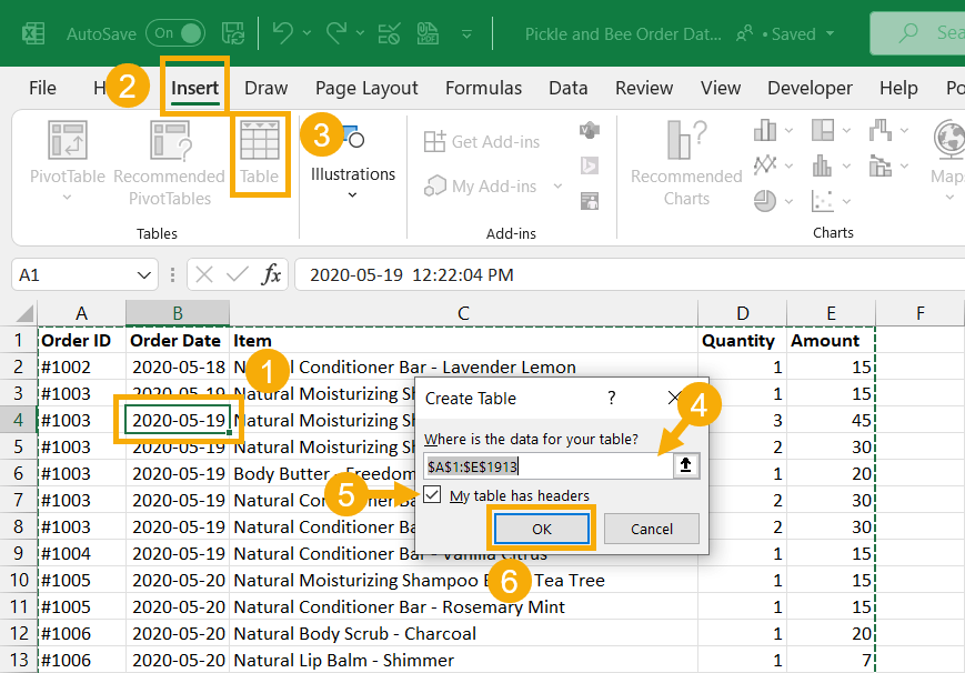
1. Select any cell inside your dataset.
2. Go to the Insert tab.
3. Click on the Table command.

This will open up the Create Table menu and you should see a green dashed line around your data to indicate what data will be included in the table.

4. Make sure Excel has correctly identified the full range of your data. You can adjust this using the selection toggle with the up arrow.
5. Check the My table has headers option. This ensures the first row will be placed in the table headings.
6. Press the OK button.

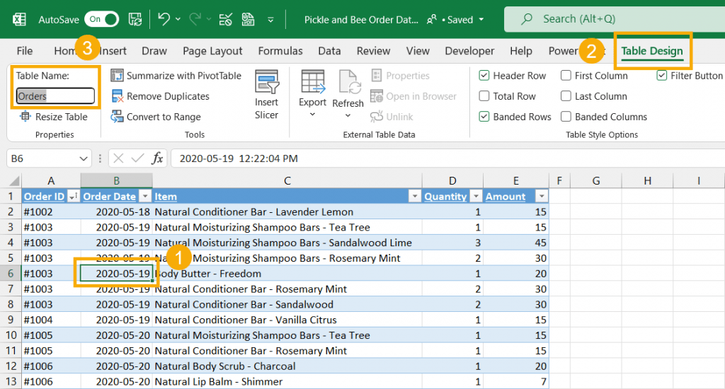
Your data is now in an Excel Table. It will be very obvious as tables come with nice formatting that is automatically applied.

You should now give your table a meaningful name instead of the generic Table1 name.

1. Select a cell inside your table.
2. Go to the Table Design tab. This is a contextual tab and will only appear when you have the active cell inside a table.
3. Type a new name into the Table Name input and press Enter.

You will now be able to reference this table name as the source data for your pivot tables.

Insert a Pivot Table with the Insert Tab

The Insert PivotTable command found in the Insert tab is the first method you should know about if you need to use pivot tables.

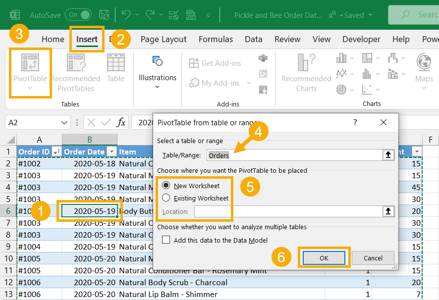
Follow these steps to insert a pivot table.

1. Select a cell inside your data.
2. Go to the Insert tab.
3. Click on the top half of the PivotTable command. You can click on the bottom half for more advanced options.
4. Make sure the Table/Range input has correctly identified your table or range for the data source.
5. Choose either a New Worksheet or an Existing Worksheet location for the new pivot table.
6. Press the OK button.

You now have a new blank pivot table in Excel!

Insert a Pivot Table with a Keyboard Shortcut

Unfortunately, there is no dedicated keyboard shortcut to insert a pivot table, but you can use the Alt hotkeys.

When you press the Alt key, you will notice various letters appear in the ribbon commands. These allow you to navigate the ribbon commands from your keyboard.

Press Alt, N, V, T to access the From Table/Range command found in the insert PivotTable options.

The insert pivot table options will be the same from this point on.

Insert a Pivot Table with Quick Access Toolbar

If you are using pivot tables a lot, then you are going to want a way to quickly access the options to insert one.

This is exactly what the Quick Access Toolbar is for!

It’s a customizable selection of frequently used commands that are always available in your Excel app.

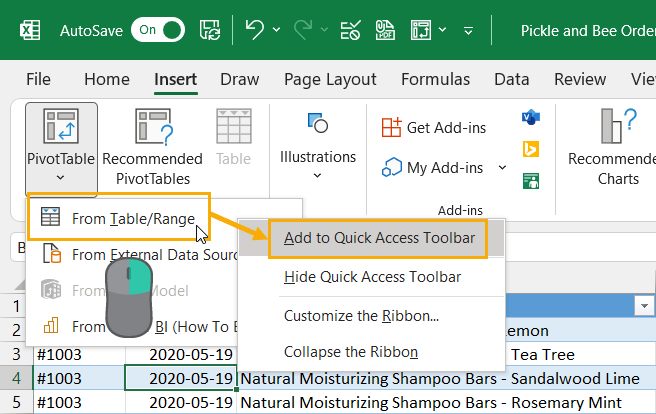
You can easily add any command found in the ribbon to your Quick Access Toolbar.

Follow these steps to add the From Table/Range command to your Quick Access Toolbar.

1. Go to the Insert tab.
2. Left-click on the bottom part of the PivotTable command.
3. Right-click on the From Table/Range option in the PivotTable submenu.
4. Choose the Add to Quick Access Toolbar options from the right-click menu.

This will add the From Table/Range command to your Quick Access Toolbar as shown above.

Anytime you need to create a pivot table you can use this command since it’s always visible!

These commands even come with Alt hotkey shortcuts based on the order they appear in the Quick Access Toolbar.

This example shows the command is placed in the 5th position of the toolbar, so you can press Alt + 5 to use the command.

Insert a Pivot Table with Table Design Tab

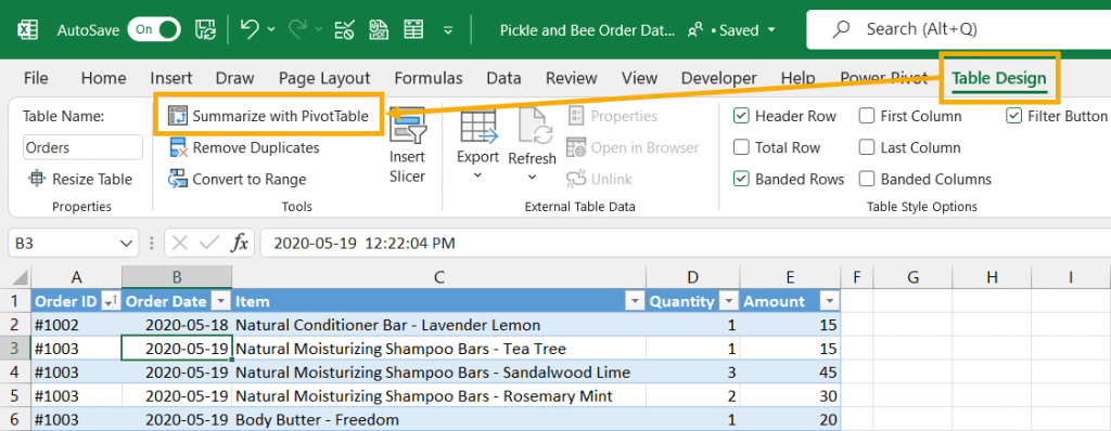
Since pivot tables are used so frequently with Excel Tables, they have included a pivot table command inside the Table Design tab.

Select a cell inside your table and the Table Design tab will appear in the ribbon.

Go to the Table Design tab and select Summarize with PivotTable.

Insert a Pivot Table with Quick Analysis

There is a really cool option called Quick Analysis. As the name suggests, it gives you quick access to various tools for data analysis.

Follow these steps to insert a pivot table with the Quick Analysis tools.

1. Select your entire dataset. Select any cell in your data and press Ctrl + A to select the entire table.

When you select your entire data set, you will see the Quick Analysis icon appear in the lower right corner.

When you click on this, it will open a menu with access to Formatting, Charts, Totals, Tables, and Sparkline tools.

You can also use the Quick Analysis keyboard shortcut to select the data and open the Quick Analysis tools. Press Ctrl + Q to open the Quick Analysis tools. This can also be achieved if you right-click on the table and choose Quick Analysis from the menu.

2. Click on the Quick Analysis tools icon.
3. Go to the Tables tab in the pop-up menu.
4. Select one of the PivotTable options. These give you a list of suggested prebuilt pivot tables based on your data.

You can hover over the various PivotTable options to see a preview of the pivot table that will result.

When you select any of the PivotTable options, it will insert the pivot table into a new sheet.

Insert a Pivot Table with Recommended PivotTables

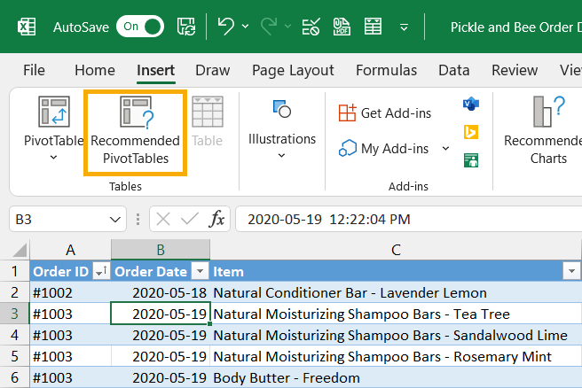
Recommended PivotTables are a great way to create a prepopulated pivot table.

This will give you a list of suggested pivot tables you can preview and then insert into your workbook.

Follow these steps to insert a recommended pivot table.

1. Select a cell inside your dataset.
2. Go to the Insert tab.
3. Click on the Recommended PivotTable command.

This will open the Recommended PivotTables menu which will show you a list of suggested pivot tables you might be interested in.

4. Select a pivot table from the left-hand side. It will show a larger preview on the right.
5. Press the OK button.

This will insert the selected pivot table into a new sheet in your workbook.

Insert a Pivot Table with Analyze Data

Analyze Data is an artificial intelligence feature that will help you spot interesting insights about your data.

It allows you to query your data with natural language questions and also provides a selection of pivot table summaries and visuals to highlight trends and patterns.

Follow these steps to use the Analyze Data feature.

1. Select a cell in your data.
2. Go to the Home tab.
3. Click on the Analyze Data command.

This will open the Analyze Data window pane on the right side.

1. You can ask questions about your data using natural language.
2. You can select from suggested questions about your data.
3. There is a list of pivot tables and visuals in the Discover Insights section.

You’ll see various pivot tables available in the Discover Insights section which you can insert into the workbook.

You can easily spot the pivot tables as they will have a prominent Insert PivotTable button in the lower-left corner.

Click on the Insert PivotTable button and it will be added to a new sheet in your workbook.

Insert a Pivot Table with Table/Range Query

Power Query is a data extraction and transformation tool available in Excel, Power BI, and a few other Microsoft products.

Your data might not come in the exact format you need before you can analyze it inside a pivot table. But you can reshape your data using Power Query and then load it directly into a pivot table.

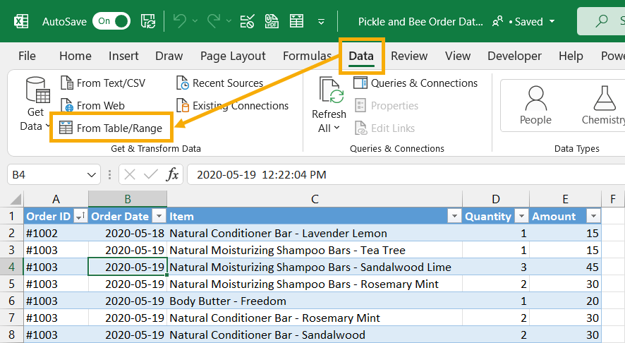
Follow these steps to load your data into Power Query.

1. Select a cell inside your data source.
2. Go to the Data tab.
3. Click on the From Table/Range command in the Get & Transform Data section.

This will open up the Power Query editor in a new window. You’ll be able to apply any sort of transformation inside the Power Query editor.

When your data is in the required format, you can then load it directly to a pivot table.

4. Go to the Home tab in the Power Query editor.
5. Click on the lower half of the Close & Load button.
6. Select Close & Load To from the options.

This will close the Power Query editor and an Import Data menu will pop up.

7. Select PivotTable Report from the loading options.
8. Choose where to load the pivot table. You can choose a location in an Existing worksheet or a New worksheet.
9. Press the OK button.

Now your transformed data will be available directly inside a pivot table.

This is a great option for adding new calculated columns to your reports!

Insert a Pivot Table with VBA

You might be looking for a way to automate building your pivot table reports.

This is where VBA programming may assist you in automating the procedure.

VBA is the scripting language built into Excel and will allow you to automate your time-consuming reporting activities.

Press Alt + F11 on your keyboard to open the VBA code editor.

Go to the Insert menu in the VBA code editor and choose Module from the drop-down list. This will create a new module where you can add your VBA code.

Sub InsertPivotTable()

ActiveWorkbook.PivotCaches.Create(SourceType:=xlDatabase, SourceData:= _
    "Orders", Version:=7).CreatePivotTable TableDestination:="Sheet1!R1C7", _
    TableName:="myPivotTableReport", DefaultVersion:=7


With ActiveSheet.PivotTables("myPivotTableReport")
    .PivotFields("Item").Orientation = xlRowField
    .AddDataField ActiveSheet.PivotTables("myPivotTableReport") _
        .PivotFields("Amount"), "Sum of Amount", xlSum
    .PivotFields("Sum of Amount").NumberFormat = "$#,##0"
End With

End Sub

You can paste the above code into the editor.

It will create a pivot table named myPivotTableReport with the Item column in the Rows area and the Amount column as a sum in the Values area. The Amount column will also get a currency format applied.

Press Alt + F8 to open the Macro dialog box where you can run your code from.

Insert a Pivot Table with Office Scripts

There is also another option for automating your report solutions.

The latest version of Excel for Microsoft 365 includes a new TypeScript based programming language called Office Scripts.

The new Office Script language is now available in Microsoft 365 business plans and may be used from the online web version of Excel.

Open Excel Online and go to the Automate tab, then click on the New Script button to open the Office Script editor.

This will open the script editor on the right side of the Excel window with a blank script.

You can click on the generic name given to the script and rename it with a descriptive name so you can easily find and run it later.

function main(workbook: ExcelScript.Workbook) {
	let orders = workbook.getTable("Orders");
	let selectedSheet = workbook.getActiveWorksheet();
	// Add a new pivot table on selectedSheet
	let newPivotTable = workbook.addPivotTable("myPivotTableReport", orders, selectedSheet.getRange("H1"));
	// Add pivot fields to newPivotTable
	newPivotTable.addRowHierarchy(newPivotTable.getHierarchy("Item"));
	newPivotTable.getRowHierarchy("Item").setPosition(0);
	newPivotTable.addDataHierarchy(newPivotTable.getHierarchy("Amount"));
	newPivotTable.getDataHierarchy("Sum of Amount").setPosition(0);
}

The above code will create a new pivot table from the Orders table and populate it with the Item and Amount field.

Click the Run button to run the script and create a pivot table.

Conclusions

Pivot tables are a fundamental tool for data analysis in Microsoft Excel, and there are many ways to insert pivot tables.

There are options to insert blank pivot tables as well as suggested prebuilt pivot tables.

Options like Recommended PivotTables and Quick Analysis tools can even suggest pivot tables that might interest you based on your dataset.

Analyze Data takes things a step further and can create pivot tables based on natural language questions you ask.

Power Query can import data from external sources, or transform your data to a proper state ready for use in a pivot table. It also allows you to conveniently load the results directly to a pivot table.

You can also automate your pivot table report creation using either VBA or Office Scripts. The possibilities for automating your reporting are endless with these tools.

Which method for inserting pivot tables do you prefer? Do you know any other ways to create pivot tables? Let me know in the comments below!