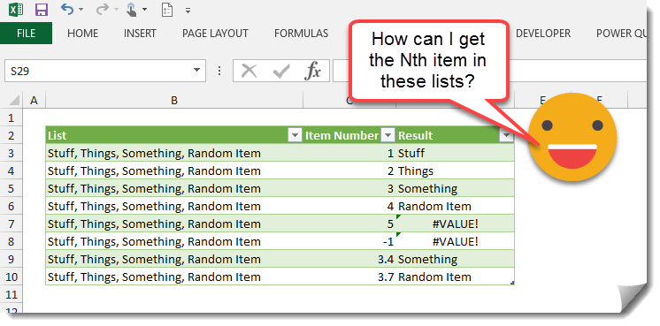
Let’s say you have a column of data and in each cell you have a text string which is a list of items separated by a comma. Something like the below table.

How can you get the Nth item from that list? One solution would be to use text to column and actually separate out each list into different columns then use an INDEX function on those column. The problem with this is in the process you’ve destroyed the original list and it’s now across many different columns. A simpler solution might be to create a user defined function in VBA for this.

Function INDEXLIST(strList As String, strSeparator As String, lngIndex As Long) As String

Dim ListArray() As String

ListArray() = Split(strList, strSeparator)

INDEXLIST = ListArray(lngIndex - 1)

End Function

This code takes advantage of the visual basic Split function to do the “heavy listing” for us in separating our list into an array, then all we need to do is call the Nth array element.

Syntax

=INDEXLIST(List,Separator,Index)

• List (required) – This is the list of delimited items.
• Separator (required) – This is the delimiter that separates the items in the list.
• Index (required) – This is the item index number which you want to return.

With this code we can obtain our Nth item from the list with this formula.

=INDEXLIST(B3,", ",C3)

Things to note about the INDEXLIST function.

• If we input an index number greater than the number or items in the list or less than the number of items in the list the function will return a #VALUE! error.
• If we use a non integer number, the function will round this to the nearest integer and return that item from the list.

A Formula Solution

It is possible to get the Nth item in a list using Excel’s built-in formulas but the solution I found is definitely not as elegant.

• Use the SUBSTITUTE function to replace the N-1th occurrence of the separator “, ” with a character that is likely to not be used in any of the items in your list, CHAR(1) should be unlikely to appear in any data. Now we can use the FIND function to find the position of this CHAR(1) character. We repeat this logic on the Nth occurrence of the separator “, “.
• Use IFERROR function to take care of when N is too big or too small.
• Use LEN and MID function to return the text between these to separators.

=SUBSTITUTE(MID(B3,IFERROR(FIND(CHAR(1),SUBSTITUTE(B3,", ",CHAR(1),C3-1)),1),IFERROR(FIND(CHAR(1),SUBSTITUTE(B3,", ",CHAR(1),C3)),LEN(B3)+1)-IFERROR(FIND(CHAR(1),SUBSTITUTE(B3,", ",CHAR(1),C3-1)),1)),", ","")

It definitely isn’t pretty, but it works.